Munich Personal RePEc Archive
Comparative Study of Static and
Dynamic Neural Network Models for
Nonlinear Time Series Forecasting
Abounoori, Abbas Ali and Mohammadali, Hanieh and
Gandali Alikhani, Nadiya and Naderi, Esmaeil
Islamic Azad University central Tehran Branch, Iran., University of
Tehran, Faculty of Economics., Islamic Azad University, Department
of Economics Science and Research Branch, khouzestan-Iran.,
University of Tehran, Faculty of Economics.
12 October 2012
Online at
https://mpra.ub.uni-muenchen.de/46466/
Comparative Study of Static and Dynamic Neural Network Models for Nonlinear Time Series Forecasting
Abbas Ali Abounoori
Assistant Professor, Islamic Azad University central Tehran Branch, Iran Email: [email protected]
Hanieh Mohammadali
MA in Economics, Faculty of Economics, University of Tehran, Iran, Email: [email protected]
Nadiya Gandali Alikhani
MA in Economics, Islamic Azad University, Department of Economics Science and Research
Branch, khouzestan-Iran. Email:[email protected].
Esmaeil Naderi1
MA student in Economics, Faculty of Economics, University of Tehran, Iran, Email: [email protected]
Abstract
During the recent decades, neural network models have been focused upon by researchers due to their more real performance and on this basis different types of these models have been used in forecasting. Now, there is this question that which kind of these models has more explanatory power in forecasting the future processes of the stock. In line with this, the present paper made a comparison between static and dynamic neural network models in forecasting the return of Tehran Stock Exchange (TSE) index in order to find the best model to be used for forecasting this series (as a nonlinear financial time series). The data were collected daily from 25/3/2009 to 22/10/2011. The models examined in this study included two static models (Adaptive Neuro-Fuzzy Inference Systems or ANFIS and Multi-layer Feed-forward Neural Network or MFNN) and a dynamic model (nonlinear neural network autoregressive model or NNAR). The findings showed that based on the Mean Square Error and Root Mean Square Error criteria, ANFIS model had a much higher forecasting ability compared to other models.
JEL Classification: G14, G17, C22, C45, C60.
Key Words: Forecasting, Stock Market,dynamicNeural Network, StaticNeural Network.
1. Introduction
Due to the importance of financial markets, any changes in these markets will impose a major
impact on the economy (Colombage, 2009). On the other hand, different changes such as
economic, social, cultural and political will affect markets leading to total confusion of the
investors, mistrust of the performance of the market, existence of asymmetric information
1
and, thereby, loss of the public confidence in the markets (Zhou and Sornette, 2006).
Therefore, over the past few decades, in order to create the optimized conditions for
allocating financial resources and evaluating the performance of risk management, the
accurate forecasting of the price changes of financial assets has attracted the attention of
researchers and policy-makers (Cox and Loomis, 2006). The classical methods such as
regression and structural models, despite their relative success in forecasting the variables,
have not produced desired results, according to researcher, because these methods generally
rely on information obtained from historical events. Mainly because the economic and
financial issues in stock market lead to the formation of complex and non-linear relations, the
use of flexible non-linear models, such as neural network models, in modeling and
forecasting the market indexes can yield impressive results (Aladag et al., 2009). On the
other hand, the use of flexible nonlinear models, such as neural network models, is a response
to the lack of consensus on rejection or acceptance of the efficient markets hypothesis.
Despite the complexity of these methods in the process of pricing, they have the ability to
forecast the future prices with acceptable error. So far, there have been several published
results on forecasting stock market prices. Melin et al. (2012), Gursen et al. (2012), Soni
(2011), Dase and Pawar (2010), Jibendu (2010), Li and Liu (2009), Pritam (2008),
Thenmozhi (2006) examined the stock market in different regions of the world using artificial
neural network models. Also, Sahin et al. (2012), Georgescu and Dinucă (2011), Mehrara et
al. (2010), Tong-Seng (2007), Ghiassi et al. (2006), Sheta and Jong (2001) forecasted the
time series using multilayer feed-forward neural network (MFNN), Nonlinear Neural
Network Auto-Regressive model with exogenous inputs (NNARX), and Adaptive
Neuro-Fuzzy Inference Systems (ANFIS) methods. The striking point in all those studies is that,
different models of neural network have a very high accuracy in forecasting the market in
comparison with the classical models.
Generally, the first step in forecasting a series is its potential predictability. Therefore,
checking the “efficient market hypothesis” or, in other words, the predictability of stock
return using the available information is of a lot of significance. In general, "efficient market
hypothesis" was proposed because of the inability to forecast the stock price due to influence
of various factors (Garanjer and Timmermann, 2004).According to the efficient market
hypothesis, prices in the stock market follow a random walk process. Because of the fast flow
of information in the market and its impact on the stock price, stock return cannot be
forecasted based on past changes in the prices (Cootner, 1964).The efficient market
impossible in a stable economy, many of the investors would be able to earn unlimited profits
(Garanjer and Timmermann, 2004). Many studies have been done on the efficiency of stock
markets most of which have found evidence of inefficiency of these markets. It should be
noted that, although a poor efficacy in the stock market has been verified in some studies,
however, due to the random appearance of the stock indexes, a specific nonlinear process can
be realized. Therefore, in such circumstances, these indicators are inefficient, and no
distinction can be found, based on the linear test, between this feature and random walk
model (Scheinkman and Lebaron, 1989; Hou et al, 2005; Abhyankar et al, 1995).
The present study is an attempt to, first, compare the static and dynamic neutral network
models, which have been used in this study and, second, to find which of these models can
make a more accurate forecast the return of Tehran Stock Exchange (TSE). For this purpose,
daily time series data were used from 25/3/2009 to 22/10/2011 (616 observations) out of
which 555 observations (about 90% of the observations) were used for modeling and 60 for
out-of-sample forecasting. Thus, before modeling the stock market index, based on the
variance ratio test and BDS, efficient market hypothesis test will be examined. If the
hypothesis is rejected, the BDS test will examine the linearity or non-linearity of the variables
to ensure the possibility of using neutral network models in forecasting these variables. In
line with this, then a brief overview will be made of the types of neural network models used
in this study and their associated properties.
2. Methodology
2.1. Neural Network Models
Despite its novelty, Artificial Intelligence (AI) has obtained the attention of scholars and
researchers. Different types of artificial neural networks attempt to emulate the human mind
or the learning process using computational methods, automate the process of knowledge
acquisition from data and solve great and complex problems. Artificial neural networks have
many applications such as data classification, function approximation, forecasting, clustering,
and optimization (Ripley, 1996; Krose, 1996) .Using artificial neural networks has many
considerable advantages; first, neural networks have a high similarity with the human
nervous system, and unlike the traditional methods, they are data-driven self-adaptive
methods, which have only few assumptions for the problems. In other words, they are
model-free; second, in addition to their high-speed information processing due to parallel
processing, neural networks have a very high generalizations; finally, because neural
networks have more comprehensive and more flexible functional forms compared to the
models are distributed parallel processes with natural essence, and their main feature is the
ability to model a complex non-linear relation without any presuppositions about the essence
of the relationships between the data. There are two types of neural networks: dynamic and
static networks (Deng, 2013; Chiang et al. 2004; Tsoi and Back, 1995). Static networks, such
as Adaptive Neuro-Fuzzy Inference Systems and Multi-layer Feed-forward Neural Network,
have no feedback, and the outputs are calculated directly based on their connection with
Feed-forward inputs. But in dynamic neural networks, such as nonlinear neural network
autoregressive (NNAR), the outputs depend on the current and past values of inputs, outputs,
and the network structure.
2.2. Static Neural Network Models
2.2.1. Feed-Forward Neural Network Models
The simplest form of a neural network has only two layers, output layer and input layer. The
networks act as an input-output system. In these systems, to calculate the value of the output
neurons, the value of the input neurons is checked by a transfer function or activator. Besides
the input and output layers, the multi-layer neural networks use the hidden layer because it
will improve the performance of the networks. First Rumelhart et al. in 1986 and since then
many authors, such as Nielson (1987), Cybenko (1989), Funahashi (1989), Hornik et al.
(1990), and White (1992), have demonstrated that Feed-forward neural network with one
logistic activation function in the hidden layerand one linear activation function in the output
neuroncan approximate any function with the desired accuracy.
2.2.2. Fuzzy Neural Network Models
The theory of the fuzzy set was introduced in 1965 by Lotfi Zadeh. Reasoning or fuzzy logic
is a powerful method with wide applications for problem solving in industrial control and
information processing. This method provides a simple way of drawing definite result from
weak, indefinite, and vague data. The most important feature of the Fuzzy method is its
ability to work with approximate data and find explicit solutions. When the pattern of
uncertainty, due to the inherent variability or uncertainty, is beyond randomness, the theory
of the fuzzy set is an appropriate method for the analysis of complex systems and decision
processes. Unlike classical logic, which requires a deep understanding of a system, precise
questions, and explicit numerical values, fuzzy logic allows us to model the complex systems
(Wanous et al, 2000). In general, fuzzy logic has three distinct stages: first, Fuzzification,
which converts the numerical data in the real-world to the fuzzy numbers; second,
Defuzzyfication, that includes the inverse transformation of obtained fuzzy numbers to the
numerical data in the real-world (Tsipouras et al, 2008).
2.3. Dynamic Neural Network Models
These models have numerous applications in different areas such as forecasting financial
markets, communication systems, power systems, classification, error detection, recognizing
voices, and even in genetics. One of the most frequently used models among dynamic neural
network models is the NNAR model. This model is developed by adding an AR process to a
neural network model. Dynamic neural network (NNAR) has a linear and a nonlinear section;
its nonlinear section is estimated by a Feed-Forward artificial neural network with hidden
layers and its linear section includes an autoregressive model (AR). The general form of the
NNAR neural network model is:
(3) )] ( ),..., 2 ( ), 1 ( ), ( ),..., 2 ( ), 1 ( ), ( [ ) ( ˆ y
u y t y t y t n
n t u t u t u t u f t
Y
In this formula, f represents a mapping performed by the neural network. The input for the network includes two u(t) exogenous variables (input signals) and target values (the lags of the output signals). The numbers for nuand
y
n include output signals and actual target values
respectively which are determined by the neural network (Trapletti et al., 2000).
The main advantage of using this model is that it is able to make more accurate long-term
forecasts under similar conditions in comparison with the ANN model (Taskaya and Caseym
2005). The training approach in these models, which is consistent with Levenberg-Marquardt
(LM) Training (Levenberg, 1944 and Marquardt, 1963) and the hyperbolic tangent activation
function, is built on Error-Correction Learning Rule and starts the training process using
random initial weights (Matkovskyy, 2012; Giovanis, 2010; Rosenblatt, 1961). After
determining the output of the model for any of the models presented in the training set, the
error resulting from the difference between the model output and the expected values is
calculated and after moving back into the network in the reverse direction (from output to
input), the error is corrected.
3. Empirical Results
In this study, the performance of static and dynamic neural networks in forecasting Tehran
Stock Exchange dividend price index and cash return was compared. The abbreviations for
the used variables in this paper include: TEDPIX (Tehran Stock Exchange dividend and price
index), which indicates the price index and cash return, and dlted, which represents the return
of the TSE. On this basis, the predictability of the related index will be examined by variance
3.1. Examining predictability of the return of TSE
In this section, in order to explain the reasons for using non-linear models, two tests will be
analyzed; first, the non-randomness (and consequently predictability) of stock return series
will be considered using the Variance Ratio Test and then its non-linearity will be examined
using the BDS test.
3.1.1. Variance Ration test (VR Test)
This test (Lo and Mac Kinlay's, 1988) is used to examine whether the behavior of the
components of stock return series is Martingale. In this test, when the null hypothesis is
rejected, it can be concluded that the tested series will not be i.i.d. Overall, rejection of the
null hypothesis in the VR test is indicative of the existence of linear or nonlinear effects
among the residuals or the time series variable under investigation (Bley, 2011).
Table 1: The results of VR test in stock series
Test Probability Value
Variance ratio test 0.000 6.38
Source: Findings of Study
The results of the above test show that there is no evidence that the mentioned series (and the
lag series) is Martingale; thus, the process of the data is not random. Accordingly,
predictability of this series is implied in this way. The interesting point is that one cannot find
out whether the data process in the stock return series is linear or non-linear as suggested by
the results of this test, but can conclude that it is non-Martingale and predictable (Al-Khazali
et al, 2011).
3.1.2. BDS test
This test which was introduced in 1987 by Brock, Dechert and Scheinkman (BDS) acts based
on the correlation integral which tests the randomness of the process of a time series against
the existence of a general correlation in it. For this purpose, the BDS method first estimates
the related time series using different methods. Then it uses correlation integral to test the
null hypothesis on the existence of linear relationships between the series. Indeed, rejection
of the null hypothesis indicates the existence of non-linear relationships between the related
time series.(Briatka, 2006).
The statistics of this test (correlation integral) measures the probability that the distance
between the two points from different directions in the fuzzy space is less than and like the
fractal dimension in the fuzzy space when there is an increase in , this probability also
) ( ] ) ( ) ( [ ) ( , , 1 , 2 1 , T m m T T m T m C C T
BDS . In this equation, m,T()is an estimation of the
distribution of the asymptotic standardCm,T()C1,T()m. If a process is i.i.d, the BDS
statistics will be asymptotic standard normal distribution. In this equation, if the BDS
statistics is large enough, the null hypothesis will be rejected and the opposite hypothesis on
the existence of a non-linear relationship in the process under investigation will be accepted
(Moloney and Raghavendra, 2011). This test can be usefully applied for assessing the
existence of a non-linear relationship in the observed time series. The results of this test have
[image:8.595.140.461.297.368.2]been provided in Table 2.
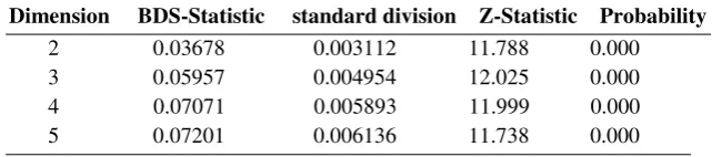
Table 2: The results of BDS test in the stock return series
Dimension BDS-Statistic standard division Z-Statistic Probability
2 0.03678 0.003112 11.788 0.000 3 0.05957 0.004954 12.025 0.000 4 0.07071 0.005893 11.999 0.000 5 0.07201 0.006136 11.738 0.000
Source: Findings of Study
As it can be seen in Table 2, the null hypothesis, that means non-randomness of the stock
return series, is rejected. So, this indicates the existence of a nonlinear process in the stock
return series (there can also be a chaotic process as well). It is worth mentioning that
whenever randomness of a series is rejected in more than two dimensions in the results of
BDS test, the probability of the nonlinearity of this series will be high (because the opposite
hypothesis is not clear in this test). So, this test can be a corroborative evidence of
nonlinearity of the stock return series. Ergo, by confirming predictability and also
nonlinearity of the related time series during the research, nonlinear models, i.e., ANN,
ANFIS and NNARX can be used for forecasting.
3.2. Estimating static models 3.2.1. Estimating MFNN model
Considering the large importance of network architecture, in this part before different types
of feed-forward neural network models, some points related to the network architecture will
be mentioned. First, in order to find the optimal number of neurons, an attempt was made to
evaluate different networks with different neurons using coding in MATLAB software.
Therefore, 2 to 20 neurons were evaluated in two- and three-layered networks; each one was
trained 30 times and in order to compare their performance, the errors in the test data which
number of neurons was found to be 8 and the optimal number of layers was determined to be
2. Furthermore, from among different algorithms, Traincgp had the best performance.
Another point to be mentioned after designing the network is the use of 5 lags of the
dependent variable and also a dummy variable (the criterion for selecting them was the
abnormal shocks to the time series under investigation in a way that the shocks greater than 3
standard deviations were regarded as the abnormal shocks) were considered as the input
variables to the model. Based on this structure, the related variable was forecasted (see Table
[image:9.595.138.492.250.303.2]3 for the results).
Table 4. Estimation of different MFNN models
Rows Models MSE RMSE
1 MFNN (5lagofdlted) 2.63*10^-5 5.13*10^-3
2 MFNN (5lagofdlted&DUMMY) 1.94*10^-5 4.41*10-3
Source: Findings of Study
As shown in Table 3, the results of these models are indicative of a desirable performance in
terms of having fewer forecasting errors considering the dummy variables.
3.2.2. Estimating ANFIS model
The modeling method used in ANFIS is similar to other system-recognizing techniques. In
the first stage, a parametric system is considered as the assumption and then input and output
data are collected in the form which is applicable in ANFIS. Then this model can be used for
training the FIS model. Generally, this kind of modeling has a suitable performance when the
data applied to ANFIS for training the membership function parameters include all the
features of the FIS model.
Adaptive Neuro-Fuzzy Inference System has a similar performance to neural networks. Due
to characteristics of this system, first the data must be converted to its fuzzy form or
normalized and then the fuzzificated data are reread into the ANFIS toolbox and finally based
on the different FIS functions (including psigmf, dsigmf, pimf, gauss2mf, gaussmf, gbellmf,
trapmf and trimf), the best function will be selected.
For selecting the type of FIS function in the ANFIS model, the following procedure was
followed. Due to the large volume of the data, each function was executed for 50 inputs
(which have been selected randomly) and the real values and output values of the network
will be obtained. Then the errors related to each function were calculated and finally the best
the present study, two Gaussian FIS functions (gaussmf and gauss2mf) have the least number
of errors and consequently the highest level of accuracy (gaussmf showed a better (though
not significant) performance). After selecting the best FIS function, the optimal network
estimated (trained) and obtained the output values of the system (the simulated values or
out-of-sample forecasting). Therefore, based on the gaussmf fuzzy inferencing system, the
number of forecasting errors of the fuzzy neural network will be estimated in out-of-sample
forecasting of the stock return series in two different AFFIS models, one having five lags of
the dependent variable and the other having five lags as well as the dummy variable which
includes the structural breaks in the stock return series during the period under investigation
[image:10.595.129.472.303.367.2](see Table 4 for the results).
Table 4. Estimation of Forecasting Criteria by Using ANFIS
Rows Models MSE RMSE
1 ANFIS (5lagofdlted) 2.01*10^-5 4.48*10^-3
2 ANFIS (5lag of dlted& DUM) 1.47*10^-5 3.83*10^-3
Source: Findings of Study
As shown in Table 4, the results of the fuzzy neural network with the input data of five lags
and the dummy variable, are more desirable in terms of the fewer forecasting errors
compared to models with five lags of dependent variable (it should be noted that considering
the fact that the validation data are not considered in the fuzzy neural networks, this value
was set as zero in other models and for testing the performance of different models, the test
data were only used).
3.3. Estimation of dynamic model
As mentioned, the first step in modeling nonlinear models based on neural networks is
"network architecture". Therefore, before comparing different NNAR and NNARX models,
the architecture of dynamic neural network should be explained.
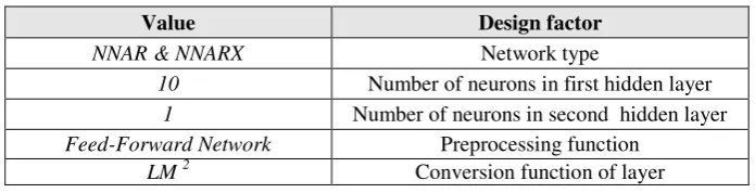
Table.5. Network Architecture Design factor Value
Network type
NNAR & NNARX
Number of neurons in first hidden layer
10
Number of neurons in second hidden layer
1
Preprocessing function
Feed-Forward Network
Conversion function of layer
LM 2
2
[image:10.595.124.472.614.703.2]Based on the network architecture that was defined in Table4, estimation and comparison of
different NNARX models are offered .As in the previous models, a dummy variable has been
[image:11.595.131.467.158.371.2]used as the input variable.
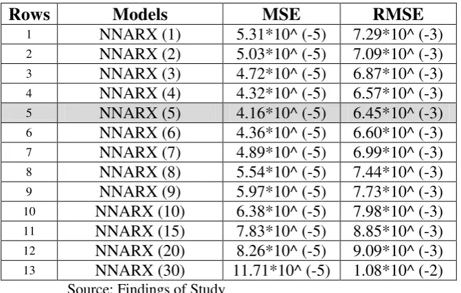
Table 6: Estimation of Forecasting Criteria by Using NNARX
Rows Models MSE RMSE
1 NNARX (1) 5.31*10^ (-5) 7.29*10^ (-3)
2 NNARX (2) 5.03*10^ (-5) 7.09*10^ (-3)
3 NNARX (3) 4.72*10^ (-5) 6.87*10^ (-3)
4 NNARX (4) 4.32*10^ (-5) 6.57*10^ (-3)
5 NNARX (5) 4.16*10^ (-5) 6.45*10^ (-3)
6 NNARX (6) 4.36*10^ (-5) 6.60*10^ (-3)
7 NNARX (7) 4.89*10^ (-5) 6.99*10^ (-3)
8 NNARX (8) 5.54*10^ (-5) 7.44*10^ (-3)
9 NNARX (9) 5.97*10^ (-5) 7.73*10^ (-3)
10 NNARX (10) 6.38*10^ (-5) 7.98*10^ (-3)
11 NNARX (15) 7.83*10^ (-5) 8.85*10^ (-3)
12 NNARX (20) 8.26*10^ (-5) 9.09*10^ (-3)
13 NNARX (30) 11.71*10^ (-5) 1.08*10^ (-2)
Source: Findings of Study
As shown in Table 5, the NNARX(5) model (using ten lags of the stock return index and the
dummy variable introduced) has had the best performance in comparison with other models
based on the MSE, and RMSE criteria.
3.4. Comparing the performance of models in accuracy of forecasts
In general, MSE and RMSE are the most commonly used criteria for comparing different
models in accurate forecasting of the results. In many studies, the RMSE criterion used as a
measure of fitting accuracy of models and includes all the features of the MSE criteria
including taking into consideration the outlier data and comparing the accuracy of models as
well as showing the error differences because it is the square root of MSE (Swanson et al,
2011).
Table 7: The results of comparison of the models
Rows Models MSE RMSE
1 MFNN (5lagofdlted&DUMMY) 1.94*10^-5 4.41*10-3 2 ANFIS (5lag of dlted & DUM) 1.47*10^-5 3.83*10^-3
3 NNARX (5) 4.16*10^ (-5) 6.45*10^ (-3)
Source: Findings of Study
Therefore, on the basis of the mentioned criteria, we will compare the accuracy performance of the models used in this study. The results of comparison have been presented in Table 7. As shown in Table 7, ANFIS static neural network model has fewer forecasting errors in
[image:11.595.147.509.614.685.2]have more acceptable performances than MFNN model in forecasting the return of Tehran
Stock Exchange index.
4. Conclusions
Basically, one of the most important economic theories in the field of financial markets is
related to the unpredictability of the changes in the price index of the stock market which is
known as random walk hypothesis. Forecasting models which have been developed for the
stock prices are, in fact, a challenge against this hypothesis and attempt to show that the
future trend of prices can be forecasted with an acceptable number of errors despite the
complications involved in the price movements. One of these models is the static and
dynamic nonlinear neural network models. These models have been rather successful in
forecasting the variables that have a very complicated process.
In this study, the dynamic neural network autoregressive model and also static fuzzy neural
network models (ANFIS) and multi-layer feed-forward neural network model (MFNN) were
used for forecasting the return of Tehran Stock Exchange index. The results presented in
Table 8 show that ANFIS model has made a more accurate forecast of stock return series.
After this model, NNARX and MFNN had a better performance in forecasting this variable
respectively. These results were not unexpected because the results of previous studies (e.g.,
Mukerji et al, 2009; Dorum et al, 2010; Kamali and Binesh, 2013) had also shown the
superiority of this model (ANFIS).
It should be noted that staticity of ANFIS and MFNN models and also dynamicity of NNAR
and NNARX models are due to the inherent features of these models and on this basis, in this
study we compared the performance of these models in forecasting TSE. In other words, the
method of analysis used in this study univariable (technical) analysis. Therefore, it can be
suggested that in future studies this method can be used in forecasting other economic
variables (such as gold price, oil price, exchange rate, etc.) as well as in multivariable
(fundamental) analysis.
Finally, the ANFIS neural network method can be introduced to policy-makers and
macro-economic decision makers as an appropriate method for making more accurate forecasts and
also to investors to help them make profits by assisting them in making good investment
decisions via more efficient forecasts made by this model.
Abhyankar, A.H., Copeland, L.S., Wong, W. (1995). Uncovering Nonlinear Dynamics
Structure in Real-Time Stock Market Indexes. Journal of Business and Economic Statistics
15(1), PP. 1-14.
Aladag, H.A., Egrioglu, E., Kadilar, C. (2009). Forecasting Nonlinear Time Series with a
Hybrid Methodology. Applied Mathematic Letters, 22, PP. 1467-147.
Al-Khazali, O.M., Pyun, C.S., Kim, D. (2012). Are Exchange Rate Movements Predictable in
Asia-Pacific Markets? Evidence of Random Walk and Martingale Difference Processes,
International Review of Economics and Finance 21(1), PP. 221–231.
Bley, J. (2011). Are GCC Stock Markets Predictable?. Emerging Markets Review 12(3), PP.
217–237.
Briatka, L. (2006). How Big is Big Enough? Justifying Results of the i.i.d Test Based on the
Correlation Integral in the Non-Normal World. Working Paper Series, Charles University,
ISSN. 1211-3298, 308, PP. 1-34.
Brock, W.A., Dechert, W.D., Sheinkman, J.A. (1987). A Test of Independence Based on the
Correlation Dimension. Working paper, University of Wisconsin at Madison, University of
Houston, and University of Chicago, 8702, PP. 1-38.
Chiang, Y. M., Chang, L. Ch., Chang, F.J. (2004). Comparison of static-feedforward and
dynamic-feedback neural networks for rainfall–runoff modeling. Journal of Hydrology,
290(3–4), PP. 297-311.
Colombage, S. (2009). Financial Markets and Economic Performances: Empirical Evidence
from Five Industrialized Economies. Research in International Business and Finance 23(3),
PP.339-348.
Cootner, H. (1964). The random character of stock market prices. M.I.T. Press,
Cox, J.E., Loomis, D.G. (2006). Improving Forecasting through Textbooks-A 25 Year
Review. International Journal of Forecasting 22(3), PP. 617-624.
Cybenko, G. (1989). Approximations by superpositions of sigmoidal functions. Mathematics
of Control, Signals, and Systems 2(4), PP. 303-314.
Dase, R.K., Pawar, D.D. (2010). Application of Artificial Neural Network for stock Market
Predictions: A review of literature. International Journal of Machine Intelligence 2(2),
pp.14-17.
Deng, J. (2013). Dynamic Neural Networks with Hybrid Structures for Nonlinear System
Identification. Engineering Applications of Artificial Intelligence 26 (1), PP. 281–292.
Dorum, A., Yarar, A. Sevimli, M. F. Onüçyildiz, M. (2010). Modelling the rainfall-runoff
data of susurluk basin, Expert Systems with Applications 37(9), PP. 6587-6593.
Funahashi, K. I. (1989). On the Approximate Realization of Continuous Mappings by Neural
Networks. Neural Networks 2(3), PP. 183–192.
Gallant A.R. White, H. (1992). On Learning the Derivatives of an Unknown Mapping with
Multilayer Feedforward Networks. Neural Networks 5, PP. 129-138.
Georgescu, V. Dinucă, E. C. (2011). Evidence of Improvement in Neural-Network Based
Predictability of Stock Market Indexes through Co-movement Entries. Recent Advances in
Applied & Biomedical Informatics and Computational Engineering in Systems Applications,
11th WSEAS International Conference on Applied Informatics and Communications,
Florence, Italy, PP.412-417.
Ghiassi, M., Zimbra, D. K. Saidane, H. (2006). Medium term system load forecasting with a
dynamic artificial neural network model. Electric Power Systems Research 76(5), PP.
Giovanis, E. (2010). Application of Feed-Forward Neural Networks Autoregressive model
with Genetic Algorithm in Gross Domestic Product Prediction, World Academy of Science,
Engineering and Technology 64. pp. 638-664.
Granger, C.W.J., Timmermann, A. (2004). Efficient market hypothesis and forecasting.
International Journal of Forecasting 20(1), PP. 15–27.
Guresen, E., Kayakutlu, G., Daim, U. T. (2011). Using Artificial Neural Network Models in
Stock Market Index Prediction. Expert Systems with Applications 38(8), PP. 10389-10397.
Hornik, K., Stinchcombe, M., White, H. (1990). Universal Approximation of an Unknown
Mapping and its Derivatives Using Multilayer Feedforward Networks, Neural Networks 3(5),
PP. 551-560.
Hou, k., Moskowitz, T.J. (2005). Market Frictions, Price Delay and the Cross-Section of
Expected Returns, Review of Financial Studies 18(3), pp. 981- 1020.
Mantri, J. K., Gahan, P., Nayak, B.B. (2010). Artificial neural networks- An application to
stock market volatility. International Journal of Engineering Science and Technology 2(5),
pp 1451-1460.
Kamali, R., Binesh, A. R. (2013). A comparison of neural networks and adaptive neuro-fuzzy
inference systems for the prediction of water diffusion through carbon nanotubes.
Microfluidics and Nanofluidics 14(3-4), PP. 575-581.
Krose, B., Smagt, P. (1996). An introduction to neural network. The University of
Amsterdam. Eighth edition.
Lee, T.H., White, H., Granger, C.W.J. (1992). Testing for Neglected Nonlinearity in
Time-Series Models: A Comparison of Neural Network Methods and Standard Tests. Journal of
Econometrics 56(3), PP. 269-290.
Levenberg, K. (1944). A Method for the Solution of Certain Nonlinear Problems in Least
Li F., Liu, C. (2009). Application Study of BP Neural Network on Stock Market Prediction.
Ninth International Conference on Hybrid Intelligent Systems 3, pp: 174-178, IEEE.
Lo, A. W., MacKinlay, C. (1988). The Size and Power of the Variance Ratio Tests in Finite
Samples: A Monte Carlo Investigation. Journal of Econometrics 40, pp. 203-238.
Lotfi, A. Z. (1965). Fuzzy sets. Information and Control 8(3), PP. 338–353.
Lotfi, A. Z. (1965). Fuzzy sets and systems. In: Fox J, editor. System Theory. Brooklyn, NY:
Polytechnic Press, PP. 29–39.
Marquardt, D. W. (1963). An Algorithm for Least Squares Estimation of Nonlinear
Parameters. Journal Society Industrial Applied Mathematics 11(2), pp. 431-441.
Matkovskyy, R. (2012). Forecasting the Index of Financial Safety (IFS) of South Africa using
neural networks, MPRA Paper 42153, University Library of Munich, Germany.
McClelland, J.L., Rumelhart, D.E., Hinton, G.E. (1986). The appeal of parallel distributed
processing. In Parallel Distributed Processing: Foundations 1, pp.3-44.
Mehrara, M., Moeini, A., Ahrari, M. Ghafari, A. (2010). Using Technical Analysis with
Neural Network for Prediction Stock Price Index in Tehran Stock Exchange. Middle Eastern
Finance and Economics 6(6), PP. 50-61.
Melin, P., Soto, J., Castillo, O., Soria, J. (2012). A new approach for time series prediction
using ensembles of ANFIS models. Expert Systems with Applications 39(3), PP. 3494-3506.
Moloney, K., Raghavendra, S. (2011). Testing for Nonlinear Dependence in the Credit
Default Swap Market, Economics Research International, Article ID 708704, PP. 1-11.
Mukerji, A., Chatterjee, C., Raghuwanshi, N.S. (2009). Flood Forecasting Using ANN,
Neuro-Fuzzy, and Neuro-GA Models. Journal of Hydrologic Engineering, 14(6), PP.
Nielsen, H. (1987). Kolomogorr’s Mapping Neural Network Existence Theorem, In IEEE
First Annual International Conference on Neural Networks 3, PP. 11-14.
Olmedo, E. (2011). Is there chaos in the Spanish labour market?.Chaos, Solitons & Fractals
44(12), PP.1045-1053.
Charkha, P. R. (2008). Stock Price Prediction and Trend Prediction using Neural Networks.
First International Conference on Emerging Trends in Engineering and Technology, pp:
592-594, IEEE.
Ripley, B.D. (1996). Pattern Recognition and Neural Networks, Cambridge University Press.
Rosenblatt, F. (1961). Principles of Neurodynamics: perceptrons and the theory of brain
mechanisms. Spartan Press, Washington.
Sahin, S., Tolu, M.R., Hassanpour, R. (2012). Hybrid expert systems: A survey of current
approaches and applications. Expert Systems with Applications 39(4), PP. 4609-4617.
Scheinkman, J., Lebaron, B. (1989). Nonlinear dynamics and stock returns. Journal of
business 62(3), PP. 311-337.
Sheta, A. F., Jong, K. D. (2001). Time-series forecasting using GA-tuned radial basis
functions. Information Sciences 133(3–4), PP. 221–228.
Soni, S. (2011). Applications of ANNs in Stock Market Prediction: A Survey. International
Journal of Computer Science & Engineering Technology 2(3), pp. 71-83.
Stinchcombe M., White, H. (1992). Using Feedforward Networks to Distinguish Multivariate
Populations. Proceedings of the International Joint Conference on Neural Networks 1,
pp.788-793.
Taskaya-Temizel, T., Casey, M.C. (2005). A Comparative Study of Autoregressive Neural
Thenmozhi, M. (2006). Forecasting Stock Index Returns Using Neural Networks. Delhi
Business Review 7(2), pp. 59-69.
Tong-Seng Q. (2007). Using Neural Network for DJIA Stock Selection. Engineering Letters
15(1). pp 15-31.
Trapletti A., Leisch, F., Hornik, K. (2000). Stationary and integrated autoregressive neural
network processes. Neural Computation 12(10), pp. 2427-2450.
Tsipouras, M., Exarchos, T.P., Fotiadis, D. (2008). Automated Fuzzy Model Generation
Through Weigh and Fuzzification Parameters' Optimization. International Conference on
Fuzzy Systems, PP. 2186-2193.
Tsoi, A. Ch., Back, A. (1995). Static and dynamic preprocessing methods in neural networks.
Engineering Applications of Artificial Intelligence 8(6), PP. 633–642.
Wanous, M., Boussabaine, A.H. Lewis, J. (2000). Bidno bid: a parametric solution.
Construction Management and Economics, 18(4), PP. 457-466.
White, H. (1992). Nonparametric Estimation of Conditional Quantiles Using Neural
Networks. In Proceedings of the Symposium on the Interface. New York: Springer-Verlag,
PP. 190-199.
Zhou, W., Sornette, D. (2006). Fundamental Factors versus Herding in the 2000–2005 US
Stock Market and Prediction. Physica A: Statistical Mechanics and its Applications 360(2),