http://www.scirp.org/journal/ojs ISSN Online: 2161-7198
ISSN Print: 2161-718X
Does Missing Data in Studies of Hard-to-Reach
Populations Bias Results? Not Necessarily
Anneliese C. Bolland
1, Sara Tomek
2, John M. Bolland
11Institute for Social Science Research, The University of Alabama, Tuscaloosa, Alabama, USA
2Department of Educational Studies in Psychology, Research Methodology, and Counseling, The University of Alabama, Tusca-loosa, Alabama, USA
Abstract
Missing data are always an issue in community-based longitudinal studies, call-ing into question the representativeness of samples and bias in conclusions, the research has generated. This may be due to the difficulty of implementing ran-dom sampling procedures in these studies and/or the inherent difficulty in sam-pling hard-to-reach segments of the population being studied. In fact, the ability to accurately study hard-to-reach populations in light of potential bias created by missing data remains an open question. In this study, missing data are de-fined as both failure to interview potential research participants identified in the sampling frame and failure to retain enrolled research participants longitudi-nally. Using the sample from the Mobile Youth Survey, a multiple-cohort, lon-gitudinal study of adolescents living in highly impoverished neighborhoods in Mobile, Alabama, we examined sample representativeness and dropout to de-termine whether missing data led to a nonrepresentative, and therefore, biased sample. Results indicate that even though random procedures are not strictly used to draw the sample, (a) the sample appears to be largely representative of the population that was studied, and (b) attrition is largely uncorrelated with characteristics of those who dropped out. This suggests that it is possible to study with validity hard-to reach populations in community settings.
Keywords
Hard-to-Reach Populations, Missing Data, Representativeness, Community-Based Research
1. Introduction
In research, some units of the analysis are more difficult to study than others. In survey research, where people are the units of analysis, some people (or more
gen-How to cite this paper: Bolland, A.C., Tomek, S. and Bolland, J.M. (2017) Does Missing Data in Studies of Hard-to-Reach Populations Bias Results? Not Necessarily. Open Journal of Statistics, 7, 264-289.
https://doi.org/10.4236/ojs.2017.72021
Received: January 25, 2017 Accepted: April 23, 2017 Published: April 26, 2017 Copyright © 2017 by authors and Scientific Research Publishing Inc. This work is licensed under the Creative Commons Attribution International License (CC BY 4.0).
http://creativecommons.org/licenses/by/4.0/
erally, groups of people with certain characteristics) are more difficult to study than others, and the term “hard-to-reach” has been used to invoke the resources needed to sample, recruit, and secure participation from individuals with these characteristics [1]. This may be due to their geographical or physical location, or to their social and economic situation [2]; these populations have also been described as “vulnerable” or “hidden” (although see [3], for a critique of these terms).
1.1. Hard-to-Reach Populations
Lambert and Wiebel [4] note that hard-to-reach populations might benefit most from knowledge about them. For example, racial minorities or ethnicities and people of low socioeconomic status (SES), who have been described as hard-to- reach [5][6][7], experience poorer health status [8][9] and poorer educational achievement [10][11][12] than non-minorities and people of higher SES.
Several factors may account for the difficulty of conducting research on these populations. For remote or geographically isolated populations, traveling to con- duct the research, coupled with possible language and cultural barriers, may be prohibitively expensive (for examples, see [2]). However, even research using easi-ly-identified local populations in the United States (e.g., inner-city adolescents) can be difficult.
The result is missing data, and despite best intentions of researchers, missing data are common in survey research involving hard-to-reach populations. This may take either (or both) of two forms: (a) lack of participation by cases identified in the sampling frame (or that would have been identified had the sampling frame been known) and targeted for recruitment; and (b) participant dropout in longitu-dinal studies (A third form of missing data, failure to answer specific questions in a survey, will not be addressed here; indeed, others argue that this form of missing data is “little more than a nuisance” [13]). Although they are typically discussed as different issues, (a) and (b) are two sides of the same coin: failure to obtain data from targeted research participants either at the point of initial recruitment or at the point of longitudinal follow up. Missing data does not, by itself, pose a threat to the validity of study results. However, when reasons for missingness are correlated with variables to be studied, selection bias results and threatens validity.
Consider, for example, how missing data might occur in a study inner-city ado-lescents. Inner-city neighborhoods are, by definition, impoverished; and given the overlap of poverty and race/ethnicity in the U.S. [14][15], they are heavily popu-lated by racial and ethnic minorities. Some have studied the “hard-to-reach” na-ture of the Black American research experience (e.g., [16][17][18]). And several studies have demonstrated lower general levels of trust among people of low SES and racial/ethnic minorities [19][20], including distrust of researchers (see [21]). Thus, response rates may be low in research conducted in inner-city neighbor-hoods.
(either at enrollment or follow up) once a sampling frame has been established. Perhaps even more problematic is the violence and victimization that is often common in inner-city neighborhoods [23] [24]; this may lead researchers to simply forego studying inner-city residents, or target neighborhoods with less violence, given the risk of injury to members of the research team. Alternatively, researchers may choose to study inner-city residents in safe environments (e.g., schools, clinics) or using safer research venues (e.g., telephone or on-line sur-veys); yet, each of these approaches risks missing significant and important seg-ments of the population (e.g., students prone to chronic absenteeism or who have dropped out of school; adults who do not have working phones).
Beyond the risks of selection bias in studies that focus on hard-to-reach pop-ulations, a more insidious problem involving exclusion of underrepresented po- pulations has been noted [25] [26]. The National Institutes of Health require underrepresented populations (i.e., women and people of color) to be included in studies it funds [27]. While this acknowledges the problem, it is unclear whether it solves the problem. Vulnerability is nested, particularly within hard- to-reach populations. As noted, poverty tends to be nested within race, as are high residential mobility rates. Poor health is further nested within race, largely because of poverty. Social isolation is likely nested within all of these conditions as well. Thus, a mandate to include underrepresented populations does not guarantee that the most vulnerable members of these disadvantaged populations will be included in research. And as a result, even studies of disadvantage may to be biased, with important negative consequences.
1.2. Missing Data: The Problem and Approaches to Address It
Of course, the easiest way to address missing data is to avoid it. Community- based participatory research [28] [29] [30], participatory action research [31] [32], and similar approaches [33] have been suggested a way to accomplish this. These designs involve the community of interest in the study from the point of original study inception (including choice of research questions and wording of survey questions), and the generated buy-in from members of the community make their participation more likely. However, this approach is limited by the fact that many study designs cannot be changed to reflect community input; moreover, even with high levels of community buy-in, missing data is inevitable.identified and recruited but who do not participate) are either MAR or MCAR and therefore ignorable. On the other hand, if these cases are MNAR, the sample is not representative. The concept of ignorability has been used most typically for dropout in longitudinal studies, but it is equally applicable to enrollment and representativeness (e.g., in a representative sample, missingness is ignorable).
Of course, it is difficult (if not impossible) to determine definitively whether or not the outcome or predictor variables are related to missingness, since by de-finition they are not measured for missing cases. While empirical means of ex-ploring whether missing data are ignorable have been developed, (e.g., [36][37]), they are strictly exploratory; they often rely on tenuous assumptions about the missing observations; they are conceptually and mathematically inaccessible to most researchers; and they have not been incorporated into any statistical analysis software. Some additional papers have developed procedures to analyze datasets with non-ignorable data (e.g., [38] [39][40]; however, these typically also make assumptions about the data and are not available through data analysis software. As an alternative, many papers (e.g., [41][42][43]) that use multiple imputation or maximum likelihood to accommodate missing data justify their decision based on papers that have logically (with some empirical support) examined whether the ignorability assumption is plausible. The paper most often used for this purpose is by Graham and colleagues [13], who argue that missing data in school-based stu-dies are seldom MNAR; others (e.g., [44]) are not so sanguine.
Graham and colleagues [13] use a combination of data analysis and thought experiment to reach their conclusion. The empirical component of their paper uses a common practice of estimating the impact of missing data based on tem-porally proximal observations as proxy measures of unobserved data; based on this approach, they found little evidence that the missing data in their study were MNAR. While perhaps the best available substitute for the true values of unob-served data, they are not the same—particularly for vulnerable populations, where the vagaries of life reduce consistency of attitudes, beliefs, and behaviors across time [45] [46]. Graham and colleagues’ thought experiment considers multiple random factors that might affect school attendance, and hence partici-pation in a school-based survey. While their assumptions very likely hold for non-poverty samples, they are less likely to hold for inner-city samples, where the effects of poverty (e.g. residential mobility; household stress; poor health) may influence school attendance. These consequences of poverty are not uni-versal within this population, however; nor are they constant across time for any given case. Thus, the effects of poverty may manifest themselves for any given student at any given time as risk behavior and missing data. That is, the greater the poverty, and the harder-to-reach the population, the greater the threat to ig-norability of missing data.
for treating missing data as ignorable. Moreover, the conclusion reached by Graham and colleagues is limited to school-based studies and does not necessar-ily apply to community-based studies. All of these issues raise a critical question: Can research be conducted with hard-to-reach populations without selection bias?
2. The Present Study
The present study addresses this question through the analysis of Mobile Youth Survey (MYS) data; the MYS was a community-based longitudinal study of po-verty and adolescent risk conducted in inner-city community-based sample in Mobile, Alabama. As is typical of such a study of this type, the sampling frame was poorly defined and high rates of missing data occurred. However, the study was able to access complete public school records for both study participants and potential participants. Thus, auxiliary data were available for both observed and missing cases each year of the study. This information is important, in that it extends the findings of Graham and colleagues [13] to community-based studies of hard-to-reach populations; in doing so, it provides researchers conducting similar studies with additional results that can be used in considering whether missing data in their studies are ignorable. Second, information can be used by researchers without access to auxiliary data to support assumptions that must be made concerning whether or not missing data are ignorable.
The aim of this study is to determine whether systematic differences exist be-tween the sample of students who (a) enrolled in the MYS (E) and those who did not, (b) participated in the MYS during any given year (P) and those who did not, and (c) were retained as MYS participants during consecutive waves of data collection (R) and those who were not. In the following notation, i denotes a person (or case), while j and k denote years (or waves) in the longitudinal data collection sequence. We define participation as a matrix P, where pij = 1 if per-son i participated in the MYS during year j. We define enrollment as a vector e, where ei= 1 if pij = 1 for any j and ei= 0 if pij = 0 for every j. Generally speaking,
E allows us to examine the representativeness of the sample, while P allows us to examine within-case year-to-year variability in representativeness. We define wave-to-wave retention as a matrix R (which varies by adjacent data waves j and
k) where rijk= 1 if pij = 1 and pik = 1; rijk= 0 if pij = 1 and pik = 0; and rijkis unde-fined if pij = 0 or i fails to meet the inclusion criteria (see the Methods Section) for either year j or year k). R allows us to examine whether missing data due to dropout are informative. In conducting these analyses, we examine how both demographic (i.e., age, sex, race) and functional (i.e., cognitive and behavioral) variables are related to missingness.
3. Methods
3.1. Mobile Youth Survey
in poverty, where the median household income was $31,445 [47]. Prichard, the second largest city in the Mobile MSA, borders Mobile to the north. In 2000, 83.3% of its residents were Black American and 44.1% of this population lived in poverty, with a median household income of $19,544 [47].
3.2. Study Sample
A total of 8708 adolescents enrolled in the MYS between 1998 and 2007; this constitutes the core sample for the study, although noted in the Inclusion sec-tion, the final sample size is somewhat smaller. In 1998, the initial wave of MYS data collection was conducted in the 13 most impoverished neighborhoods in the Mobile MSA; 98% or respondents reported that they were Black). In 1990, the population in these neighborhoods was over 95% Black; median household income was $5190 and the poverty rate was 73% [48].
When it began, the sampling frame for the MYS was 10 - 18 year-old adoles-cents who lived in these neighborhoods, with the goal of recruiting the entire el-igible population of elel-igible adolescents. This goal was pursued using both an ac-tive (random) and passive (non-random) recruitment strategy (see [49] for addi-tional detail). Since a large number of MYS participants were not contacted through active recruitment and the final sample fell well short of the full popula-tion, the MYS sample cannot be viewed as randomly selected.
In 1998, 1771 respondents completed the MYS. The response rate is difficult to calculate because a definitive census of the sampling frame was not available. However, a conservative estimate of a response rate among those actively re-cruited is 60% [50]. During each subsequent year, previous participants who re-mained age-eligible were actively recruited to participate, even if residential mo-bility took respondents beyond one of the 13 target neighborhoods. By 2005, 38.8% of the MYS participants lived outside of the original target neighbor-hoods. Residential relocation tended to be clustered, leading to the identification of “expansion neighborhoods”.
Research participants were paid for their time each year ($10 between 1998 and 2004; $15 after 1994). The MYS typically required between 60 and 90 mi-nutes completing.
3.3. Inclusion Criteria
other source (i.e., records from the Mobile County Juvenile Court, the Mobile Housing Authority, the Mobile Police Department’s Family Intervention Team program for at-risk youths; the Lexis Nexispublic records database), and we as-sume that these cases are bogus (some adolescents may have given fake names so as to be allowed to participate multiple times and receive multiple cash incen-tives for their participation). Thus, we obtain an effective match to MCPSS records of approximately 95%. An analysis of Family Intervention Team pro-gram records shows that only five of 656 (0.7%) MYS enrollees in the propro-gram attended non-public schools, and none were home schooled. This is consistent with national statistics, showing that (a) fewer than 5% of Black American youths living in households with annual incomes less than $20,000 attended private schools [51], and (b) the homeschooling rate for youths living in poverty is 0.7% [52]; the lower private and home school estimates for the MYS sample may reflect the extreme levels of poverty in which MYS enrollees live.
The second inclusion criterion involves age. Public school records provide more-or-less complete data for adolescents living in the MYS neighborhoods, with one major caveat: Alabama law allows students to drop out of school when they turn 16; thus age is used as an exclusionary factor in this study. While age was limited by the MYS’ design (eligibility of participants limited to 10 to 18 years old), in the current study, data are limited to students aged 10 through 15. Because students are legally required to attend school through the age of 15, a neighborhood sample of youths under age 16 (adjusted for students who do not attend private schools and are not home schooled) and the MCPSS census of students under age 16 are coincident. Because there is little home-schooling and private-school attendance in these neighborhoods, the adjustment makes little difference. Beyond age 15, however, the neighborhood youth census and the MCPSS census begin to deviate, due to the possibility of school dropout; since dropouts are more likely to engage in risk behaviors [53][54] and hold deviant attitudes or beliefs [55] [56] than non-dropouts, including youths aged 16 through 18 in the study would introduce bias. Age eligibility was calculated by date of birth from MCPSS records. Students were eligible if they turned 10 by August 15 of the school year and were not eligible if turned 16 after May 16th of the school year.
in terms of their characteristics.
Based on these inclusion criteria, the final sample consisted of 7142 MYS enrollees and 25,442 students who were not MYS enrollees but who lived in MYS neighborhoods.
3.4. Demographic Characteristics
Demographic variables examined in this study include sex, race, free lunch eligi-bility status, and grade, all based on MCPSS records. Sex is straightforward, and for analysis purposes, girl = 1 and boy = 0. Race/ethnicity was identified in these records as Black, White, Asian, Native American, Hispanic, and unspecified. Overall, 99.8% of MYS enrollees were classified as Black or White; this is consis-tent with MYS self-reported race, where 99.8% also reported themselves to be Black or White. We therefore treated cases that were coded by MCPSS as Asian, Native American, Hispanic, or unspecified as missing. For analysis purposes, Black = 1 and White = 0. School lunch status was coded in the MCPSS records as free, reduced-cost, and paid, with the vast majority of MCPSS participants re-ceiving free lunches; for convenience, and because of the small number of MYS participants who were in the other two categories, the categories were combined to yield a dichotomous measure: “Free” and “Not Free” status. For analysis pur-poses, free lunch = 1 and paid lunch = 0. Free lunch status was a proxy for vul-nerability associated with low SES. For ease of interpretation, grade was centered for analysis purposes at 3rd grade = 0. Finally, 48 MYS neighborhoods were iden-tified; these were divided into two groups: original target neighborhoods and expansion neighborhoods.
3.5. Functional Characteristics
In this study, functional characteristics include school achievement, as indicated by Stanford Achievement Test (SAT) percentile ranks, and by violation of school code-of-conduct; each is a component of MCPSS student records.
Student achievement in Alabama was assessed annually using the SAT. The SAT, 9th edition was completed by 3rd through 11th grade students through the 2001-2002 academic year. Beginning in spring 2003, the SAT, 10th edition, was administered annually to 3rd through 8th grade students. While results for the SAT 9th edition are not directly comparable to results from the SAT 10th edition, this study compares students within year; our use of standardized percentile scores across years makes such comparisons less problematic. The reading and math subscales of the SAT are used in these analyses.
3.6. Analysis Plan
In this study, we conduct statistical analyses to determine whether demographic and functional characteristics affect enrollment, participation, and retention. We also examine the magnitude of each observed effect to determine how much it might potentially have biased the MYS sample. Each of the ten waves of MYS data was paired to the subsequent school year (e.g., 1998 MYS (wave 1) corres-ponds to the 1998-1999 school year). While such comparisons cannot indicate whether the missing data are ignorable or non-ignorable (no analysis can strictly demonstrate this), they can provide an indication of whether the MYS sample is representative of the larger neighborhood population from which it was drawn on indicators that reflect potential sources of bias.
Strictly speaking, a sample is representative only if its characteristics do not differ from the population in terms of specific study variables. This requirement can be relaxed to some extent, although conclusions about representativeness are stronger as the characteristics used to assess representativeness align more closely with the study variables. Thus, while representativeness does not guaran-tee MAR or MCAR, these conditions do guaranguaran-tee representativeness; but as the characteristics used to assess representativeness more closely approximate study variables, any loss of correspondence between representativeness and MAR or MCAR will have decreasing importance and can be safely ignored.
To assess whether missingness in MYS data were affected by demographic and functional characteristics (i.e., whether the MYS sample is representative of the population on these variables), models were estimated using a Generalized Esti-mating Equations (GEE) framework [57] [58], as implemented in SAS proc-genmod. Because all of the outcome variables (E, P, and R) were dichotomous, the models were estimated using a logit link function and a binomial error dis-tribution. We specified the working longitudinal correlation structure as first order autoregressive. For each outcome variable, two analyses were conducted. First (Model 1), the outcome variable was regressed on the demographic charac-teristics; second (Model 2), functional characteristics were added to the previous model. Since neighborhood is completely nested within neighborhood type, we included that nesting in the models. Because of the large number of neighbor-hoods, we treat it as a statistical control, reporting only omnibus p values de-rived from a Type 3 test for each outcome variable.
There is no general agreement on how to calculate effect sizes for GEE mod-els, so we calculated means for different levels of each characteristic as a proxy. For categorical predictors, these are least squares estimates of the probability of the outcome (e.g., enrollment) for each category of the predictor variable. For continuous predictors, these are probability estimates of the outcome variable when the predictor is one standard deviation below and above the mean, with all other variables held at their means (or modal category).
using a procedure suggested by Cohen [59]:
( )
(
1)
(
1( )
)
1 2
2 sin 2 sin
h′ = ⋅ − p − ⋅ − p .
Note that h’ is not equivalent Cohen’s measure of effect size (h) for the simple test of proportions, since h does not take into account the complexity of repeated measures or multiple covariates, nor is it meant to compare two points in a con-tinuous distribution (e.g., M ± S). Nonetheless, it provides a guide for interpret-ing the magnitude of reported effects. Cohen specifies small effect sizes in the range of h = 0.2, medium effect sizes in the range of h = 0.5, and large effect sizes in the range of h = 0.8.
4. Results
Table 1 provides descriptive statistics for the variables that structure the analyses reported in this section: enrollment, participation, and retention. Table 1(a) shows the frequency distributions for categorical variables and the means and standard deviations for continuous variables for (a) the entire sample; (b) stu-dents enrolled in the MYS; and (c) stustu-dents not enrolled in the MYS. The first thing to note is that for the total sample 107,689 observations are nested in 32,584 students. Observations consist of annual slices of data derived from school records for each student during the years that they were age eligible for inclusion in the study. New students entered the sample each year and remained in the sample until they moved to a non-MYS neighborhood or aged out of the study. Thus, students in the sample had an average of 3.30 observations. Second, it is clear that observations are not independent. Thus, the statistics reported in the table should be interpreted cautiously. But they nonetheless show that over-all, the students in the sample were overwhelmingly Black; they were evenly split between girls and boys; they were living in poverty; their performance on the SAT was well below average; and they were caught violating the MCPSS Code of Conduct with some frequency. Table 1(a) also provides a comparison of demo-graphic and functional characteristics of MYS enrollees and students living in MYS neighborhoods who were not enrolled in the MYS. It is important to rec-ognize that MYS enrollees remain in that classification each year for which MCPSS records are available for them, even if they did not actually participate in the MYS that year.
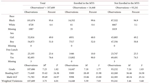
Table 1(b) shows statistics for the demographic and functional variables as a function of participatory status. Panel A is the same as Panel A in Table 1(a), since the entire sample can be divided participatory groupings. However, unlike enrollment, a student enrolled in the MYS does not automatically retain MYS par-ticipant status each year; during those years that they participated in the MYS, they were classified as MYS participants, but during those years that they did not they were classified as non-participants. This is reflected in the lower number of obser-vations for MYS participants (14,448) than for MYS enrollees (27,761).
Table 1. (a) Descriptive statistics by MYS enrollment status. (b) Descriptive statistics by MYS participation status. (c) Descriptive statistics by MYS retention status.
(a)
Total Enrolled in the MYS Not Enrolled in the MYS N = 32,584 N = 7142 N = 25,442 Observationsa = 107,689 Observations = 27,761 Observations = 79,928
Observations Percent Observations Percent Observations Percent Race
Black 101,874 95.6 27,546 99.5 74,328 94.2 White 4728 4.4 147 0.5 4581 5.8 Missing 1087 68 1019
Sex
Girl 52,816 49.0 13,182 47.5 39,634 49.6 Boy 54,873 51.0 14,579 52.5 40,294 50.4
Missing 0 0 0
Free Lunch
No 25,193 23.4 3247 11.7 21,946 27.5 Yes 82,493 76.6 24,514 88.3 57,979 72.5
Missing 3 0 3
Observations Mb Sc Observations M S Observations M S
Grade 107,686 7.23 1.82 27,760 7.07 1.77 79,919 7.28 1.83 Reading SAT 71,649 35.42 24.38 18,284 29.38 21.98 53,365 37.49 24.81
Math SAT 71,783 39.49 24.97 18,320 34.24 23.00 53,463 41.30 25.36 Weighted
Violations 107,689 3.75 6.01 27,761 4.99 7.03 79,928 3.31 5.55
aObservations indicate the number of discrete data points obtained over multiple years. Because each person potentially contributed data during multiple years. Observations ≥ N. bMean. cStandard Deviation.
(b)
Total Enrolled in the MYS Not Enrolled in the MYS Observationsa = 107,689 Observations = 14,448 Observations = 93,241
Observations Percent Observations Percent Observations Percent Race
Black 101,874 95.6 14,352 99.6 87,522 94.9 White 4728 4.4 61 0.4 4667 5.1 Missing 1087 35 1019
Sex
Girl 52,816 49.0 6931 48.0 45,885 49.2 Boy 54,873 51.0 7517 52.0 47,356 50.8
Missing 0 0 0
Free Lunch
No 25,193 23.4 1446 10.0 23,747 25.5 Yes 82,493 76.6 13,002 90.0 69,491 74.5
Missing 3 0 3
Observations Mb Sc Observations M S Observations M S
Grade 107,686 7.23 1.82 14,447 7.18 1.77 93,232 7.24 1.83 Reading SAT 71,649 35.42 24.38 9389 28.49 21.98 62,260 36.46 24.58
Math SAT 71,783 39.49 24.97 9398 33.86 23.00 62,385 40.34 25.14 Weighted Violations 107,689 3.75 6.01 14,448 5.59 7.03 93,241 3.46 5.68
(c)
Total Enrolled in the MYS Not Enrolled in the MYS Observationsa = 10,691 Observations = 7795 Observations = 2896
Observations Percent Observations Percent Observations Percent Race
Black 10,625 99.4 7754 99.7 2871 99.4 White 41 0.4 23 0.3 18 0.6 Missing 25 18
Sex
Girl 5115 47.8 3735 47.9 1380 47.7 Boy 5576 52.2 4060 52.1 1516 52.3
Missing 18 0 0
Free Lunch
No 1191 11.1 715 9.2 476 16.4 Yes 9500 88.9 7080 90.8 2420 83.6
Missing 0 0 0
Observations Mb Sc Observations M S Observations M S
Grade 10,690 7.51 1.58 7794 7.51 1.57 2896 7.53 1.59 Reading SAT 6524 27.42 21.38 4834 26.86 21.03 1690 29.02 22.28
Math SAT 6514 32.44 22.40 4819 32.19 22.18 1695 33.13 5.68 Weighted
Violations 10,691 6.24 7.68 7795 6.44 7.89 2896 5.68 7.04
aObservations indicate the number of discrete data points obtained over multiple years. bMean. cStandard Deviation.
eligible to participate in the MYS during at least one pair of consecutive years. Observations reflect MCPSS records for the second of each pair of eligible years. Students who participated during the second year were classified as retained for that year, and students who did not participate during the second year were clas-sified as not retained. Thus, the same student could be clasclas-sified in each of the two groups for different years. The number of observations is considerably smaller than for enrollment and retention (10,691 total observations for reten-tion versus 101,874 for enrollment and participareten-tion). As with Table 1(a) and Table 1(b), the statistics reported here are based on non-independent samples and should be interpreted cautiously.
4.1. Enrollment
Table 2 shows results for enrollment. For Model 1, race, lunch status, and grade level were all statistically significant predictors of enrollment. With respect to race, Black Americans were more likely to enroll in the MYS than White stu-dents (p = 0.218 versus p = 0.083). Free lunch recipients were more likely to enroll than those who did not receive free lunch (p = 0.143 versus p = 0.128). Grade level was positively related to MYS enrollment, with p = 0.221 for stu-dents one standard deviation below the mean (M − S) and p = 0.238 for students one standard deviation above the mean (M + S).
[image:12.595.56.537.83.392.2]Table 2. Determinants of MYS enrollment and associated probabilities. Mode1 l: Ŷ = b0 + b1 race (white) + b2 sex (boy) + b3 lunch (free) + b4 grade + b5 neighborhood; Mode1 2: Ŷ = b0 + b1 race (white) + b2 sex (boy) + b3 lunch (free) + b4 grade + b5 neighbor-hood+ b6 SAT (R) + b7 SAT (M) + b8 violations.
Model 1 Model 2 Estimated Probability
Effect Size Effect Parameter Parameter Estimate SEa Z p Parameter
Estimate SE Z p MeanLS b Mc − Sd M + S
Intercept b0 −1.687 0.104 −16.29 <0.001 −1.545 0.128 −12.07 <0.001
Race 0.387
White b1 −1.150 0.130 −8.86 <0.001 −1.458 0.151 −9.63 <0.001 0.083
Black 0.218
Sex 0.009
Boy b2 −0.023 0.029 −0.79 0.428 0.002 0.029 0.08 0.937 0.134
Girl 0.137
Free Lunch
Status 0.044
Not Free Lunch b3 −0.129 0.014 −9.31 <0.001 −0.153 0.019 −7.78 <0.001 0.128
Free Lunch 0.143
Neighborhood b4 <0.001 <0.001
Grade b5 0.029 0.003 9.36 <0.001 0.018 0.005 3.96 <0.001 0.221 0.238 0.040
SAT Reading b6 −0.003 0.004 −6.71 <0.001 0.251 0.227 0.056
SAT Math b7 −0.001 0.004 −3.13 0.002 0.244 0.233 0.026
School Violations b8 0.005 0.001 3.59 <0.001 0.234 0.244 0.023
aStandard Error. bLeast Squares means controlling for other variables in the equation; these have been converted to probabilities. cMean. dStandard Devia-tion.
and math SAT percentiles and school violations statistically affect the probability of MYS enrollment. For SAT percentile scores, the effect was negative. For reading, M ± S decreases from p = 0.251 for students one standard deviation be-low the reading mean to p = 0.227 for students one standard deviation above the reading mean; for math, M ± S decreases from p = 0.244 to p = 0.233. In con-trast, weighted school violations have a positive effect on enrollment, with M ± S
increasing from p = 0.234 (M − S) to p = 0.244 (M + S).
Table 2 also reports the least square means for the categorical variables (in this case, the probability of enrollment in the MYS given a particular characte-ristic and controlling for the other charactecharacte-ristics in the model); the probability of enrolling in the MYS when a given continuous characteristic is one standard below and one standard deviation above its mean; and the effect size (measured as h’). Of particular note is the small magnitude of most of the effect sizes; recall that Cohen [59] specifies small, medium, and large effect sizes as 0.20. 0.50, and 0.80). Only race (h’ = 0.387) even approaches a moderate effect size; the effect sizes of other significant predictors range between miniscule and very small (all
h’s < 0.06).
predictors of enrollment: sex × SAT reading percentile (Z = 1.98, p = 0.048) and grade × school violations (Z = 3.03, p = 0.002). In the interest of brevity, these interaction results are not included in Table 2.
4.2. Participation
By definition, participation rates are lower than enrollment rates (unless reten-tion equals unity, which was not the case in the MYS, and rarely occurs in a community-based study). Table 3 shows that in Model 1, race, free lunch status, and grade were all statistically significant predictors of participation. Black stu-dents had higher participation rates than White stustu-dents (p = 0.195 versus p = 0.015). Students receiving free lunch were more likely to participate than stu-dents who did not (p = 0.048 versus p = 0.030). And, students in higher grades were more likely to participate than those in lower grades (p = 0.119 versus p = 0.159 for students in grades one standard deviation below and one standard deviation above the grade mean, respectively).
[image:14.595.59.537.428.711.2]Model 2 shows the effects of functional characteristics on participation con-trolling for demographic characteristics. As was the case with enrollment, both reading and math SAT percentile scores were negatively associated with partici-pation. For reading, M ± S decreases from p = 0.150 for students one standard deviation below the reading mean to p = 0.122 for students one standard deviation
Table 3. Determinants of MYS participation and associated probabilities. Mode1 l: Ŷ = b0 + b1 race (white) + b2 sex (boy) + b3
lunch (free) + b4 grade + b5 neighborhood. Mode1 2: Ŷ = b0 + b1 race (white) + b2 sex (boy) + b3 lunch (free) + b4 grade + b5 neighborhood + b6 SAT (R) + b7 SAT (M) + b8 violations.
Model 1 Model 2 Estimated Probability Effect
Size Effect Parameter Parameter Estimate SEa Z p Parameter
Estimate SE Z p MeanLS b Mc − Sd M + S
Intercept b0 −3.305 0.191 −17.29 <0.001 −3.164 0.238 −13.29 <0.001
Race 0.381
White b1 −1.957 0.189 −10.38 <0.001 −1.662 0.207 −8.04 <0.001 0.015
Black 0.095
Sex 0.010
Boy b2 0.033 0.029 1.11 0.246 −0.055 0.034 −1.63 0.103 0.039
Girl 0.037
Free Lunch Status 0.094
Not Free Lunch b3 −0.497 0.027 −18.34 <0.001 −0.565 0.039 −14.46 <0.001 0.030
Free Lunch 0.048
Neighborhood b4 <0.001 <0.001
Grade b5 0.124 0.006 20.99 <0.001 0.114 0.008 13.58 <0.001 0.119 0.159 0.116
SAT Reading b6 −0.005 0.001 −6.01 <0.001 0.150 0.122 0.082
SAT Math b7 −0.002 0.001 −2.36 0.019 0.144 0.127 0.050
School Violations b8 0.017 0.001 15.12 <0.001 0.119 0.154 0.102
above the reading mean; for math, M ± S decreases from p = 0.144 to p = 0.127. Weighted school violations had a positive effect on enrollment, with M ± S in-creasing from p = 0.119 (M − S) to p = 0.154 (M + S).
Table 3 also reports estimated probability of annual participation given a par-ticular characteristic as well as the effect sizes for these characteristics. Like enrollment, race is the only variable that approaches a moderate effect size (h’ = 0.381). All other effect sizes are very small (all h’s < 0.12).
As was the case with enrollment, a supplemental version of Model 2 was also run with the twelve demographic × functional interaction terms. Two were sta-tistically significant predictors of participation: school lunch status × SAT read-ing percentile (Z = −2.53, p = 0.011) and grade × school violations (Z = 2.55, p = 0.011). These results are not reported in Table 3.
[image:15.595.59.537.428.712.2]4.3. Retention
Table 4 shows results for retention. In Model 1, race and school lunch status were statistically significant. Retention for Black students was higher than for White students (p = 0.570 versus p = 0.351), and higher for students who re-ceived free lunch than for those did not (p = 0.523 versus p = 0.396). Model 2 shows results for functional characteristics controlling for demographic charac-teristics. Here, only SAT reading percentile was a statistically significant predictor
Table 4. Determinants of MYS retention and associated probabilities. Mode1 l: Ŷ = b0 + b1 race (white) + b2 sex (boy) + b3 lunch
(free) + b4 grade + b5 neighborhood; Mode1 2: Ŷ = b0 + b1 race (white) + b2 sex (boy) + b3 lunch (free) + b4 grade + b5 neighbor-hood + b6 SAT (R) + b7 SAT (M) + b8 violations.
Model 1 Model 2 Estimated Probability
Effect Size Effect Parameter Parameter Estimate SEa Z p Parameter
Estimate SE Z p MeanLS b Mc − Sd M + S
Intercept b0 0.172 0.304 0.57 0.571 −0.107 0.431 −0.25 0.804
Race 0.443
White b1 −0.893 0.364 −2.46 0.014 −0.658 0.431 −1.53 0.127 0.351
Black 0.570
Sex 0.006
Boy b2 −0.011 0.051 −0.21 0.837 −0.022 0.067 −0.33 0.742 0.457
Girl 0.460
Free Lunch Status 0.256
Not Free Lunch b3 −0.514 0.067 −7.66 <0.001 −0.590 0.100 −5.89 <0.001 0.396
Free Lunch 0.523
Neighborhood b4 <0.001 <0.001
Grade b5 0.011 0.016 0.69 0.489 0.057 0.025 2.25 0.024 0.724 0.711 0.029
SAT Reading b6 −0.004 0.002 −1.98 0.048 0.715 0.665 0.108
SAT Math b7 0.003 0.002 1.74 0.082 0.701 0.680 0.045
School Violations b8 0.013 0.011 1.21 0.225 0.677 0.703 0.056
of retention: for students with a SAT reading percentile score one standard devi-ation below the reading mean, p = 0.715 compared with p = 0.665 for students with a SAT reading percentile score one standard deviation above the mean.
Table 4 also reports estimated probability of annual retention given a partic-ular characteristic as well as the effect sizes for these characteristics. Here, race approaches a moderate effect size (h’ = 0.443), and the effect size for free lunch status falls in the small-to-moderate range (h’ = 0.256. All other effect sizes range between miniscule and very small (all h’s < 0.11).
None of the 12 demographic × functional terms included in the supplemental analysis were statistically significant.
5. Discussion
The study of minority youths living in poverty has proven difficult, resulting in non-representative samples and high attrition rates (see [7] [16]); the result is missing data that cannot be ignored [60] [61] [62] [63]. Even when response rates are high, the possibility of bias, whether or not overtly detectable, is not eliminated [64][65].
In some studies, like those involving poverty, random sampling strategies may not be successful due to factors like high residential mobility within impove-rished populations [66] [67]. In studies like the MYS, where we attempted to study the population of adolescents living in impoverished neighborhoods, ar-guably random sampling is irrelevant; however, as the participation rate de-creases from unity, this strategy increasingly generates a convenience sample (i.e., those who chose to participate). Thus, it is important to examine missing data mechanisms that may lead to non-representativeness in all research studies, especially those involving hard-to-reach populations, because when important characteristics in the sample differ from the population, missing data are not ig-norable. We developed a protocol for doing this with the MYS, an important dataset that has been used in over 60 publications to date.
While matching sample demographic characteristics to those of the popula-tion is an important step in any study, it is seldom sufficient to demonstrate re-presentativeness; the reason is largely due to the previously-discussed nesting of vulnerability that is particularly evident in hard-to-reach populations. When re-search questions involve beliefs, attitudes, and behaviors, it is also important to determine whether the sample is representative of the population in terms of functional characteristics like cognitive abilities and behaviors. This study as-sesses the extent to which the MYS sample deviates from the population of ado-lescents living in MYS neighborhoods, in terms of their enrollment, year-to-year participation, and retention, and therefore, the extent to which missing data may be nonignorable.
sta-tistically significant results. In terms of grade, stasta-tistically different rates of MYS enrollment and participation were evident; for example, students one standard deviation below the grade mean were less likely to enroll than students one standard deviation above the mean (p = 0.221 versus p = 0.238). The difference, while statistically significant, is quite small (Δp = 0.017; h’ = 0.04). The effect for participation is also significant and also small (Δp = 0.040; h’ = 0.116). The sta-tistical significance coupled with the small effect size is likely due to the very large sample size used for these analyses (e.g., for the enrollment demographic analysis, N = 107,689 observations across 10 years), which results reduces the standard error of the estimate dramatically. We see this same outcome (a statis-tically significant estimate coupled with a small effect size) throughout the re-sults. The differences for grade, although small, may nonetheless suggest the possibility that parents of younger students were more likely to withhold consent for MYS enrollment or participation; it may also suggest the possibility that younger students were less likely to venture out of their homes and walk to the survey administration site.
Race has a significant effect on both enrollment and participation; but here, effect sizes border on robust (Δp = 0.135, h’ = 0.387 for enrollment; Δp = 0.08;
h’ = 0.381 for participation). Perhaps because very few White students lived in the MYS neighborhoods (4.4%), the perception may have developed that the MYS was a study of Black adolescents, and White adolescents largely self-se- lected out of the study. Alternatively, demographic distributions may not be geographically uniform within any given neighborhood, and there is evidence [68] that rates of enrollment and participation were higher in certain sectors of each neighborhood than in others. This was particularly the case for expanded neighborhoods, where MYS households tended to cluster on selected street blocks. We recruited most heavily on these blocks, and previous non-partici- pants were more aware of the study than adolescents living at some distance from the selected blocks. School lunch status had a significant effect on all three outcomes; effect sizes were small for enrollment (Δp = 0.015, h’ = 0.044) and participation (Δp = 0.018, h’ = 0.094), but larger for retention (Δp = 0.127, h’ = 0.256).
In the introduction, we suggested that missing data is a bigger problem in studying vulnerable and hard-to-reach populations (e.g., racial minorities, those living in poverty) than in studying populations that are not vulnerable or hard to reach. Even though our reported results suggest that the MYS sample may not be strictly representative of the population, those for race and school lunch status
run contrary to what we would expect in studying hard-to-reach populations:
would suggest. One additional explanation might argue that since MYS partici-pants were paid for their time, those living in greater poverty (i.e., receiving free lunches) would be more likely to participate. While this explanation may be par-tially valid, its importance is undermined by three factors: a) the size of the pay-ments ($10 or $15, depending on the year) were small; b) the neighborhoods were impoverished, and even those students who did not qualify for free lunch did not live in wealthy households; c) the fact that Blacks were overrepresented in the MYS, even controlling for free lunch status, suggests that the most vul-nerable adolescents in the neighborhoods chose to participate in the MYS.
Even though SES is related to cognitive ability [69] and behavior [70][71], we nonetheless expected to see a wide range of cognitive abilities and behaviors in the neighborhoods we studied; indeed, this was the case. SAT reading and math scores both ranged between the 1st percentile and the 99th percentile, and weighted school violations zero and 81 in a given year. But we found that after controlling for demographic factors, neither standardized school test scores nor behavioral violations of school codes of conduct differed in a meaningful way by enroll-ment, participation, or retention. To be sure, a number of these differences were statistically significant; for example, the SAT reading scores had a statistically significant effect on enrollment. However, the effect size was quite small (Δp = 0.024; h’ = 0.056); the largest effect size among all of the functional characteris-tics was for SAT reading on retention (Δp = 0.05, h’ = 0.108). All differences for functional characteristics showed that the most vulnerable segments of the pop-ulation (i.e., those with lower cognitive abilities; those whose behaviors violated school codes of conduct and/or resulted in disciplinary action) were oversam-pled.
Overall, demographic variables did not interact with functional variables to affect outcomes. Of the 36 variable pairs tested across three outcomes, only four results achieved statistical significance, and only one pair achieved significance across two different outcomes: the grade by school violations interaction was a significant predictor of both enrollment and participation, but not of retention (p = 0.241). Further examination showed that the effect of school violations on both enrollment and participation became increasingly positive as grade in-creased. The MYS was not conducted in schools during the school year, so school discipline (e.g., suspension) as a response to violations would not explain the effect. However, younger adolescents are more likely than older adolescents to be subject to parental monitoring and restrictive rules—rules that might pre-vent them from MYS participation. Thus adolescents who were “in trouble” (e.g., who had been disciplined for violating school rules) may well have come under even greater parental monitoring and restrictive rules, and their MYS enrollment and participation may have suffered as a consequence. But overall, demographic and functional characteristics did not interact in predicting out-comes, and it is reasonable to treat them as separate characteristics in the analy-sis.
and annual participation (0.134) are quite low, although the annual retention rate (0.729) is quite reasonable in a study of this type. In the 13 initial target neighborhoods, the enrollment and participation rates were much higher than these estimates suggest; for example, in the largest of the initial target neighbor-hoods, the 1998 participation rate was approximately 0.50, and the enrollment rate for that neighborhood was approximately 0.75 [50]. The overall much lower enrollment and participation rates for the study occur because expansion neighborhoods were added as the study progressed. Thus, the results reported here are based on all students (of appropriate ages; see the Method section for inclusion criteria) in all original and expansion neighborhoods, even though some of these neighborhoods had very few if any MYS participants during the study’s early years. It should also be noted that the expansion neighborhoods, though still more impoverished and with higher concentrations of minorities than the median neighborhood in the Mobile MSA, were, by definition not as poor as the initial target neighborhoods, and had greater racial heterogeneity.
The general conclusion, then, is that, with the exception of race (and to a less-er extent, school lunch status), the demographic and functional charactless-eristics of the MYS sample were very similar to students living in MYS neighborhoods who were not enrolled in the study. Even the racial differences in enrollment, partic-ipation, and retention and the school lunch difference in retention provide an indication that missing data was least common in the least vulnerable segment of this population. Thus, the hardest-to-reach segment of this hard-to-reach popu-lation was not only equally-likely to participate but actually even more likely to enroll, participate, and follow-up than other less-vulnerable segments of the population. In terms of the question posed earlier, we apparently were able to study this population without sampling or retention bias. It is, then, possible to reach hard to reach populations, in this case low-income minority adolescents.
We should briefly describe how we conducted the study, because that poten-tially influenced the results we were able to obtain. First, written parental sent was obtained for all participants enrollees. But we explicitly asked for con-sent for each adolescent to participate each year until he or she turned 19 (when the participant aged out). This allowed each enrollee to participate each year, whether or not direct contact with him or her or a parent/guardian occurred during that year. Word spread quickly that the MYS was in progress each year, and it was well regarded in each of the neighborhoods (to the point where study participants were overheard bragging to each other about how many times they had participated). Thus, each year many adolescents participated even though they were not individually and/or directly recruited.
neighbor-hood, and the survey became a special event in neighborhoods where special events are rare. Certainly, the fact that participants were paid for their time was important; but this rate of pay was considerably lower than what is often paid in similar studies. Surveys were also administered in the neighborhoods where each participant lived—or if that was inconvenient for the participant, in his or her home. Arguably, then, the fact that the research team was willing to go into their neighborhoods (which many of them recognized as potentially dangerous plac-es) and their homes earned a great deal of respect.
Finally, a word about the members of the research team is warranted. Each year, an internship was offered, at first to college students in Alabama, then in-creasingly to students nationally. Small stipends were provided for the interns, to cover their living expenses. But in deciding who to select for the internship (typ-ically the number of applicants outnumbered the number of available positions by a factor of three-to-four), priority was given to applicants with (a) research experience (preferably in the field) and (b) an appreciation for the effects of po-verty and a strong desire to better understand how it affects people’s lives. Thus, the interns were both very respectful of the people with whom they interacted, and they were very good listeners, learning as much from their day-to-day expe-riences in the neighborhoods and interactions with neighborhood residents as from the actual data they collected.
Strengths and Limitations
charac-teristics used in this study do not directly correspond to risk behaviors in the MYS; therefore, we cannot say with certainty that the representativeness we found extends to all cognitive, attitudinal, and behavioral domains. However, even the limited set of measures we use go well beyond what is available to ad-dress the issues of representativeness and missing data in hard-to-reach popula-tions considered by most studies.
6. Conclusions
This study suggests that researchers can conduct studies of impoverished ado-lescents without bias, so long as they carefully attend to issues of establishing le-gitimacy, respect, and trust in the communities they study. This study may also generalize to other hard-to-reach populations, although more research is needed to make this leap. Unfortunately, we do not know definitively how to establish legitimacy, respect, and trust in vulnerable communities. Our previous discus-sion suggests ways that this may be accomplished, and other papers (e.g., [2] [72][73]) explore effective ways of conducting research with hard-to-reach pop-ulations; but again, more research is needed, particularly in community-based (rather than clinical or school-based) studies.
Over 60 papers have been published using the MYS data. This study benefits those papers (and future papers that use MYS data) by suggesting that missing data in the MYS sample are largely ignorable. Our results indicate that while demographically, the MYS sample (ages 10 through 15) is not strictly represent-ative of the population, the deviations do not suggest that those who were eligi-ble, but did not participate, did so for largely-ignorable reasons. Moreover, sur-vey research literature shows lower response rates for minorities and people liv-ing in poverty. The fact that we find higher rates of enrollment and year-by-year participation for Black adolescents and those who are eligible for free lunch sug-gests that the strategy of focusing on the most at-risk segments of the MYS neighborhoods is successful and further supports the idea that the neighborhood per se is an inappropriate sampling frame. Further, results show that functional-ly, while there are significant effects for reading and math scores and for school violations, these differences are quite small and show higher enrollment, partic-ipation, and retention rates for this most vulnerable segment of the population. Thus, the results provide support for treating missing data in the MYS as ignor-able.
Acknowledgements
The research reported here was partially supported by the National Institutes of Health Office for Research on Minority Health through a cooperative agreement administered by the National Institute for Child Health and Human Develop-ment (HD30060); a grant from the Center for Substance Abuse TreatDevelop-ment, Sub-stance Abuse and Mental Health Services Administration (TI13340); a grant from the National Institute on Drug Abuse (DA017428); a grant from the Cen-ters for Disease Control and Prevention (CE000191); a grant from the National Institute for Child Health and Human Development (HD058857); The Univer-sity of Alabama; the cities of Mobile and Prichard; the Mobile Housing Board; and the Mobile County Health Department.
References
[1] Gorin, S., Hooper, C.A., Dyson, C. and Cabral, C. (2008) Ethical Challenges in Con- ducting Research with Hard to Reach Families. Child Abuse Review, 17, 275-287.
https://doi.org/10.1002/car.1031
[2] Shaghaghi, A., Bhopal, R.S. and Sheikh, A. (2011) Approaches to Recruiting “Hard- to-Reach” Populations into Research: A Review of the Literature. Health Promo-tion, 1, 1-9.
[3] Freimuth, V.S. and Mettger, W. (1990) Is There a Hard-to-Reach Audience? Public Health Reports, 105, 232-238.
[4] Lambert, E. and Wiebel, W. (1990) Introduction. In: Lambert, E. and Wiebel, W., Eds., The Collection and Interpretation of Data from Hidden Populations, National Institute on Drug Abuse Research Monograph 98, Government Printing Office, Washington DC, 1-3.
[5] Haley, D.F., Lucas, J., Golin, C.E., Wang, J., Hughes, J.P., Emel, L., et al. (2014) Re-tention Strategies and Factors Associated with Missed Visits among Low Income Women at Increased Risk of HIV Acquisition in the US (HPTN 064). AIDS Patient Care and STDs, 28, 206-217. https://doi.org/10.1089/apc.2013.0366
[6] Katz, K.S., El-Mohandes, A., Johnson, D.M., Jarrett, M., Rose, A. and Cober, M. (2001) Retention of Low Income Mothers in a Parenting Intervention Study. Jour-nal of Community Health, 26, 203-218. https://doi.org/10.1023/A:1010373113060
[7] Sullivan, C.M., Rumptz, M.H., Campbell, R., Eby, K.K. and Davidson, W.S. (1996) Retaining Participants in Longitudinal Community Research: A Comprehensive Protocol. The Journal of Applied Behavioral Science, 32, 262-276.
https://doi.org/10.1177/0021886396323002
[8] Reiss, F. (2013) Socioeconomic Inequalities and Mental Health Problems in Child-ren and Adolescents: A Systematic Review. Social Science & Medicine, 90, 24-31. [9] Nandi, A., Glymour, M.M. and Subramanian, S.V. (2014) Associations among
So-cioeconomic Status, Health Behaviors, and All-Cause Mortality in the United States. Epidemiology, 25, 170-177. https://doi.org/10.1097/EDE.0000000000000038
[10] Entwisle, D.R., Alexander, K.L. and Olson, L.S. (1994) The Gender Gap in Math: Its Possible Origins in Neighborhood Effects. American Sociological Review, 59, 822- 838. https://doi.org/10.2307/2096370
[11] Alspaugh, J.W. (1991) Out-of-School Environmental Factors and Elementary Achievement in Mathematics and Reading. Journal of Research and Development in Education, 24, 53-55.
Child-ren’s Homework: An Intervention in the Middle Grades. Family Relations, 47, 149- 157. https://doi.org/10.2307/585619
[13] Graham, J.W., Hofer, S.M., Donaldson, S.I., MacKinnon, D.P. and Schafer, J.L. (1997) Analysis with Missing Data in Prevention Research. In: Bryant, K.J., Windle, M. and West, S.G., Eds., The Science of Prevention: Methodological Advances from Alcohol and Substance Abuse Research, American Psychological Association, Washington DC. https://doi.org/10.1037/10222-010
[14] Do, D.P., Frank, R. and Finch, B.K. (2012) Does SES Explain More of the Black/ White Health Gap than We Thought? Revisiting Our Approach toward Under-standing Racial Disparities in Health. Social Science & Medicine, 74, 1385-1393. [15] Braveman, P.A., Cubbin, C., Egerter, S., Chideya, S., Marchi, K.S., Metzler, M. and
Posner, S. (2005) Socioeconomic Status in Health Research: One Size Does Not Fit All. JAMA, 294, 2879-2888. https://doi.org/10.1001/jama.294.22.2879
[16] Hatchett, B.F., Holmes, K., Duran, D.A. and Davis, C. (2000) African Americans and Research Participation: The Recruitment Process. Journal of Black Studies,30, 664-675. https://doi.org/10.1177/002193470003000502
[17] Kerkorian, D., Traube, D.E. and McKay, M.M. (2007) Understanding the African American Research Experience (KAARE): Implications for HIV Prevention. Social Work in Mental Health,5,295-312. https://doi.org/10.1300/J200v05n03_03
[18] Pottick, K.J. and Lerman, P. (1991) Maximizing Survey Response Rates for Hard-to- Reach Inner-City Populations. Social Science Quarterly,72,172-180.
[19] Merry, S.E. (1981) Urban Danger: Life in a Neighborhood of Strangers. Temple University Press, Philadelphia, PA.
[20] Ross, C.E. and Jang, S.J. (2000) Neighborhood Disorder, Fear, and Mistrust: The Buffering Role of Social Ties with Neighbors. American Journal of Community Psy- chology, 28, 401-420. https://doi.org/10.1023/A:1005137713332
[21] Yancey, A.K., Ortega, A.N. and Kumanyika, S.K. (2006) Effective Recruitment and Retention of Minority Research Participants. Annual Review of Public Health, 27, 1-28. https://doi.org/10.1146/annurev.publhealth.27.021405.102113
[22] Sampson, R.J., Morenoff, J.D. and Gannon-Rowley, T. (2002) Assessing “Neighbor- hood Effects”: Social Processes and New Directions in Research. Annual Review of Sociology, 28, 443-478. https://doi.org/10.1146/annurev.soc.28.110601.141114
[23] Peterson, R.D., Krivo, L.J. and Harris, M.A. (2000) Disadvantage and Neighborhood Violent Crime: Do Local Institutions Matter? Journal of Research in Crime and De-linquency, 37, 31-63. https://doi.org/10.1177/0022427800037001002
[24] Veysey, B.M. and Messner, S.F. (1999) Further Testing of Social Disorganization Theory: An Elaboration of Sampson and Groves’s “Community Structure and Crime”. Journal of Research in Crime and Delinquency, 36, 156-174.
https://doi.org/10.1177/0022427899036002002
[25] Odierna, D.H. and Schmidt, L.A. (2009) The Effects of Failing to Include Hard-to- Reach Respondents in Longitudinal Surveys. American Journal of Public Health, 99, 1515-1521. https://doi.org/10.2105/AJPH.2007.111138
[26] Weitzman, B.C., Guttmacher, S., Weinberg, S. and Kapadia, F. (2003) Low Re-sponse Rate Schools in Surveys of Adolescent Risk Taking Behaviours: Possible Bi-ases, Possible Solutions. Journal of Epidemiology and Community Health, 57, 63- 67. https://doi.org/10.1136/jech.57.1.63
http://grants.nih.gov/grants/funding/women_min/guidelines_amended_10_2001.ht m
[28] Belone, L., Lucero, J.E., Duran, B., Tafoya, G., Baker, E.A., Chan, D., et al. (2016) Community-Based Participatory Research Conceptual Model: Community Partner Consultation and Face Validity. Qualitative Health Research, 26, 117-135.
https://doi.org/10.1177/1049732314557084
[29] Hacker, K. (2013) Community-Based Participatory Research. Sage Publications, Thousand Oaks.
[30] Oetzel, J.G., Zhou, C., Duran, B., Pearson, C., Magarati, M., Lucero, J., et al. (2015) Establishing the Psychometric Properties of Constructs in a Community-Based Par-ticipatory Research Conceptual Model. American Journal of Health Promotion, 29, e188-e202.
[31] Chevalier, J.M. and Buckles, D. (2013) Participatory Action Research: Theory and Methods for Engaged Inquiry. Routledge, Abingdon-on-Thames.
[32] Whyte, W.F. (1989) Advancing Scientific Knowledge through Participatory Action Research. Sociological Forum, 4, 367-385.
[33] Marcellus, L. (2004) Are We Missing Anything? Pursuing Research on Attrition. CJNR (Canadian Journal of Nursing Research), 36, 82-98.
[34] Collins, L.M., Schafer, J.L. and Kam, C. (2001) A Comparison of Inclusive and Re-strictive Strategies in Modern Missing Data Procedures. Psychological Methods, 6, 330-351. https://doi.org/10.1037/1082-989X.6.4.330
[35] Schafer, J.L. and Graham, J.W. (2002) Missing Data: Our View of the State of the Art. Psychological Methods, 7, 147-177. https://doi.org/10.1037/1082-989X.7.2.147
[36] Daniels, M.J. and Hogan, J.W. (2008) Missing Data in Longitudinal Studies: Strate-gies for Bayesian Modeling and Sensitivity Analysis. Taylor & Francis, Boca Raton, FL.
[37] Molenberghs, G. and Kenward, M. (2007) Missing Data in Clinical Studies. Wiley, West Sussex, England. https://doi.org/10.1002/9780470510445
[38] Guan, Z. and Qin, J. (2017) Empirical Likelihood Method for Non-Ignorable Miss-ing Data Problems. Lifetime Data Analysis, 23, 113-135.
https://doi.org/10.1007/s10985-016-9381-0
[39] Kim, J.K. and Yu, C.L. (2011) A Semiparametric Estimation of Mean Functionals with Nonignorable Missing Data. Journal of the American Statistics Association, 106, 157-165. https://doi.org/10.1198/jasa.2011.tm10104
[40] Scharfstein, D.O., Rotnitzky, A. and Robins, J.M. (1999) Adjusting for Nonignora-ble Drop-Out Using Semiparametric Nonresponse Models. Journal of the American Statistical Association, 94, 1096-1146.
https://doi.org/10.1080/01621459.1999.10473862
[41] Bolland, J.M., Lian, B.E. and Formichella, C.M. (2005) The Origins of Hopelessness among Inner-City African-American Adolescents. American Journal of Community Psychology, 36, 293-305. https://doi.org/10.1007/s10464-005-8627-x
[42] King, D.W., Taft, C., King, L.A., Hammond, C. and Stone, E.R. (2006) Directionali-ty of the Association between Social Support and Posttraumatic Stress Disorder: A Longitudinal Investigation. Journal of Applied Social Psychology, 36, 2980-2992.
https://doi.org/10.1111/j.0021-9029.2006.00138.x
[43] McAuley, E., Elavsky, S., Motl, R.W., Konopack, J.F., Hu, L. and Marquez, D.X. (2005) Physical Activity, Self-Efficacy, and Self-Esteem: Longitudinal Relationships in Older Adults. Journal of Gerontology, 60, 268-275.
[44] Peugh, J.L. and Enders, C.K. (2004) Missing Data in Educational Research: A Re-view of Reporting Practices and Suggestions for Improvement. Review of Educa-tional Research, 74, 525-556. https://doi.org/10.3102/00346543074004525
[45] Rebellon, C.J., Manasse, M.E., Van Gundy, K.T. and Cohn, E.S. (2014) Rationalizing Delinquency: A Longitudinal Test of the Reciprocal Relationship between Delin-quent Attitudes and Behavior. Social Psychology Quarterly, 77, 361-386.
https://doi.org/10.1177/0190272514546066
[46] Rahn, W.M. and Transue, J.E. (1998) Social Trust and Value Change: The Decline of Social Capital in American Youth, 1976-1995. Political Psychology, 19, 545-565.
https://doi.org/10.1111/0162-895X.00117
[47] U.S. Census Bureau (2012) 2000 Census. https://www.census.gov/ [48] U.S. Census Bureau (2012) 1990 Census. https://www.census.gov/
[49] Bolland, K.A., Bolland, J.M., Tomek, S., Devereaux, R.S., Mrug, S. and Wimberly, J.C. (2016) Trajectories of Adolescent Alcohol Use by Gender and Early Initiation Status. Youth & Society, 48, 3-32. https://doi.org/10.1177/0044118X13475639
[50] Bolland, J.M. (2007) Mobile Youth Survey Overview. Unpublished Manuscript, University of Alabama at Birmingham, Birmingham.
[51] U.S. Census Bureau (2015) Table 8.
https://www.census.gov/topics/education/school-enrollment.html
[52] Redford, J., Battle, D. and Bielick, S. (2016) Homeschooling in the United States: 2012 (NCES 2016-096). National Center for Education Statistics, Institute of Educa-tion Sciences, U.S. Department of EducaEduca-tion, Washington DC.
[53] Freudenberg, N. and Ruglis, J. (2007) Reframing School Dropout as a Public Health Issue. Preventing Chronic Disease, 4, A107.
[54] Townsend, L., Flisher, A.J. and King, G. (2007) A Systematic Review of the Rela-tionship between High School Dropout and Substance Use. Clinical Child and Fam-ily Psychology Review, 10, 295-317. https://doi.org/10.1007/s10567-007-0023-7
[55] Chen, D., Drabick, D.A. and Burgers, D.E. (2015) A Developmental Perspective on Peer Rejection, Deviant Peer Affiliation, and Conduct Problems among Youth. Child Psychiatry & Human Development, 46, 823-838.
https://doi.org/10.1007/s10578-014-0522-y
[56] McGee, L. and Newcomb, M.D. (1992) General Deviance Syndrome: Expanded Hierarchical Evaluations at Four Ages from Early Adolescence to Adulthood. Jour-nal of Consulting and Clinical Psychology, 60, 766-776.
https://doi.org/10.1037/0022-006X.60.5.766
[57] Liang, K.Y. and Zeger, S.L. (1986) Longitudinal Data Analysis Using Generalized Linear Models. Biometrika, 73, 13-22. https://doi.org/10.1093/biomet/73.1.13
[58] Diggle, P., Heagerty, P., Liang, K. and Zeger, S. (2002) Analysis of Longitudinal Da-ta. Oxford University Press, Oxford, England.
[59] Cohen, J. (1988) Statistical Power Analysis for the Behavioral Sciences. 2nd Edition, Lawrence Erlbaum Associates, Inc., Hillsdale, NJ.
[60] Bor, W., Najman, J., O’Callaghan, M., Williams, G.M. and Anstey, K. (2001) Aggre- ssion and the Development of Delinquent Behavior in Children. Australian Institute of Criminology Trends and Issues in Crime and Criminal Justice, 207, 1-6.
[61] Buhi, E.R., Goodson, P. and Neilands, T.B. (2008) Out of Sight, Not Out of Mind: Strategies for Handling Missing Data. American Journal of Health Behavior, 32, 83- 92. https://doi.org/10.5993/AJHB.32.1.8
Im-proving Response Rates for a Hard-to-Reach Population. The Public Opinion Quar- terly, 67, 126-138. https://doi.org/10.1086/346011
[63] Way, N. and Robinson, M.G. (2003) A Longitudinal Study of the Effects of Family, Friends, and School Experiences on the Psychological Adjustment of Ethnic Minor-ity, Low-SES Adolescents. Journal of Adolescent Research, 18, 324-346.
https://doi.org/10.1177/0743558403018004001
[64] Groves, R.M. (2006) Nonresponse Rates and Nonresponse Bias in Household Sur-veys. Public Opinion Quarterly, 70, 646-675.
[65] Groves, R.M. and Peytcheva, E. (2008) The Impact of Nonresponse Rates on Non-response Bias: A Meta-Analysis. Public Opinion Quarterly,72,167-189.
https://doi.org/10.1093/poq/nfn011
[66] Lennon, M.C., Clark, W.A. and Joshi, H. (2016) Residential Mobility and Wellbe-ing: Exploring Children’s Living Situations and Their Implications for Housing Po- licy. Longitudinal and Lifecourse Studies, 7, 197-200.
https://doi.org/10.14301/llcs.v7i3.393
[67] Rosenblatt, P. and DeLuca, S. (2012) “We Don’t Live Outside, We Live in Here”: Neighborhood and Residential Mobility Decisions Among Low-Income Families. City & Community, 11, 254-284. https://doi.org/10.1111/j.1540-6040.2012.01413.x
[68] Bolland, A.C. (2012) Representativeness Two Ways: An Assessment of Representa-tiveness and Missing Data Mechanisms in a Study of an At-Risk Population. Doc-toral Dissertation, The University of Alabama, Tuscaloosa.
[69] Von Stumm, S. and Plomin, R. (2015) Socioeconomic Status and the Growth of In-telligence from Infancy through Adolescence. Intelligence, 48, 30-36.
[70] de Winter, A.F., Visser, L., Verhulst, F.C., Vollebergh, W.A. and Reijneveld, S.A. (2016) Longitudinal Patterns and Predictors of Multiple Health Risk Behaviors among Adolescents: The TRAILS Study. Preventive Medicine, 84, 76-82.
https://doi.org/10.1016/j.ypmed.2015.11.028
[71] Evans, G.W., Li, D. and Whipple, S.S. (2013) Cumulative Risk and Child Develop-ment. Psychological Bulletin, 139, 1342-1396. https://doi.org/10.1037/a0031808
[72] Bonevski, B., Randell, M., Paul, C., Chapman, K., Twyman, L., Bryant, J., et al. (2014) Reaching the Hard-to-Reach: A Systematic Review of Strategies for Improv-ing Health and Medical Research with Socially Disadvantaged Groups. BMC Medi-cal Research Methodology, 14, 42. https://doi.org/10.1186/1471-2288-14-42
[73] Faugier, J. and Sargeant, M. (1997) Sampling Hard to Reach Populations. Journal of Advanced Nursing, 26, 790-797. https://doi.org/10.1046/j.1365-2648.1997.00371.x