Exchange Rate Uncertainty and Import Demand of Thailand

Munich Personal RePEc Archive

Exchange Rate Uncertainty and Import

Demand of Thailand

Jiranyakul, Komain

National Institute of Development Administration

March 2013

NATIONAL INSTITUTE OF DEVELOPMENT ADMINISTRATION

EXCHANGE RATE UNCERTAINTY AND

IMPORT DEMAND OF THAILAND

Working Paper

Komain Jiranyakul

School of Development Economics

National Institute of Development Administration Bangkok, Thailand

Email:komain_j@hotmail.com

ABSTRACT

This study investigates the impact of real exchange rate uncertainty on import demand of Thailand. The period of study is during July 1997 to December 2011. The results from bounds testing for cointegration show that all variables are cointegrated. Even though there is no short-run impact, but the long-run negative impact of real exchange rate uncertainty on real imports is large and highly significant under the floating exchange rate regime. In the long run, a rise in real exchange rate uncertainty can improve the

country’s trade balance by substantially lowering import demand, but can harm industrial production at the same time. Therefore, stabilization of real effective exchange rate via major nominal exchange rates may deem necessary.

Key words: exchange rate uncertainty, GARCH, imports, ARDL bounds testing

INTRODUCTION

The conventional equations are used to analyze the determinants of trade flows in earlier previous studies. Two important determinants in these equations (exports and imports) are real exchange rate and real income. Warner and Kreinin (1983) use the data from 19 developing countries to identify the determinants of trade flows. They find that the impact of real exchange rate is strong on exports, but ambiguous on imports. Miles (1979) examines the impact of devaluation on trade flows, but finds that the test results are not convincing. However, the reexamination by Himarios (1989) shows that real exchange rate significantly affects trade flows. Arize and Walker (1992) employ cointegration analysis to find the determinants of import demand in Japan and find that the omission of effective exchange rate can lead to insignificant results. Tang (2004) reassesses aggregate import demand function in the ASEAN-5 economies. The results from bounds testing for cointegration show that the volume of imports, national cash flow and relative price of imports are not cointegrated in Thailand and other two ASEAN countries. Hegerty et al. (forthcoming) give a thorough review of the Marshall-Lerner condition, which states that a depreciation of real exchange rate improves trade balance, and vice versa. They find that the evidence that supports the Marshall-Lerner condition is weak.

Thailand is one of Asian countries that have liberalized trade policy. It is widely believed that import flow reacts more rapidly to trade liberalization compared to export flow. After a switching from fixed to floating exchange rate regime, the country has faced unpredictable movements in real effective exchange rate.

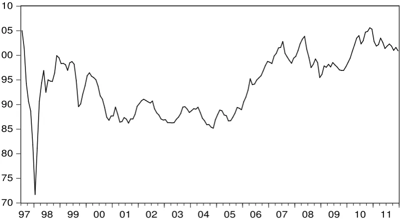
70 75 80 85 90 95 100 105 110

97 98 99 00 01 02 03 04 05 06 07 08 09 10 11

Figure 1.Index of real effective exchange rate, July 1997 to December 2011

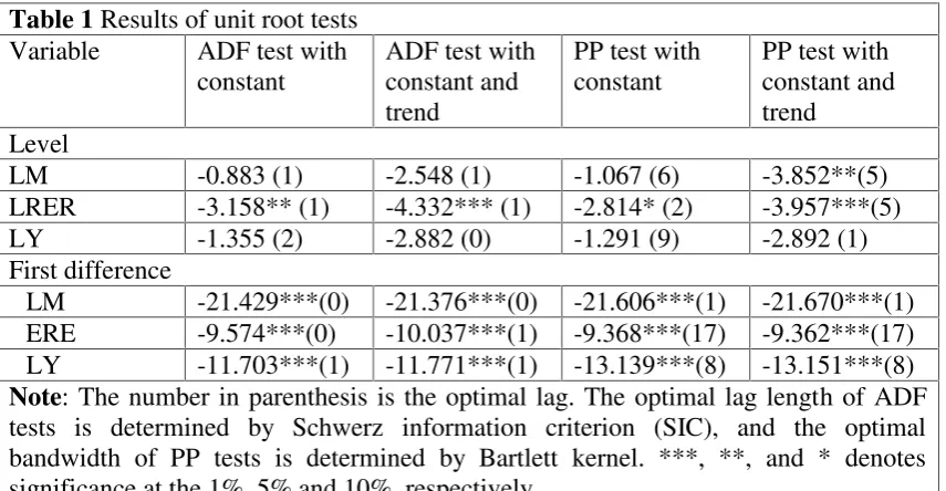
Figure 1 shows the real effective exchange rate index after Thailand adopted the floating exchange rate regime. The real effective exchange rate dropped sharply after the financial crisis and recovered in 1998. For the rest of the period the real exchange rate moved up and down with the rising trend starting from 2005 onward. The Asian financial crisis led to pronounced swings in the real effective exchange rate and thus caused Thai importers to face unavoidable uncertainty with the relative prices of imported good, especially capital equipment. Figure 2 shows the real exchange rate uncertainty.1

1

.0000 .0005 .0010 .0015 .0020 .0025 .0030 .0035 .0040

97 98 99 00 01 02 03 04 05 06 07 08 09 10 11

Figure 2. Volatility of the real effective exchange rate for Thailand

The real effective exchange rate uncertainty seemed to subside after four years of the floating exchange rate regime. However, this uncertainty might well effects real imports of the country. The results from this study are able to provide some implications regarding commercial policy that deals with trade imbalances. Whether or not revision of commercial policy is necessary, policymakers should know what factors determine the import demand function of the country, especially the impact of real exchange rate uncertainty.2 The present paper provides an evidence of long-run negative impact of real exchange rate uncertainty on real imports of Thailand under the floating exchange rate regime. The paper is organized as the following. Section 2 describes the data and empirical model. Section 3 gives empirical results, and the final section gives concluding remarks.

DATA AND METHODOLOGY

Data

Monthly data from July 1997 to December 2011 are collected from the Bank of Thailand. The data consist of real imports, real effective exchange rate, and industrial production index used as a proxy of domestic real income.3 The period of investigation is under the floating exchange rate regime, which can cause higher degree of exchange rate uncertainty (see Hassan and Wallace, 1996, Naseem, et al. 2009).

2

Arize,et al. (2008) point out the importance of this issue for countries that switched from a fixed to a flexible exchange rate regime because they can experience higher degree of exchange rate fluctuations.

3

Empirical Models for Estimations

The model used in this study relies on the international trade theory. The generalized Marshall-Lerner condition can be investigated using the import demand function that emphasizes the role of real exchange rate and real domestic income. The linear functional form for import demand is specified as

t t t

t a a LRER a LY

LM  ₀  ₁  ₂ ε (1)

where LM is the log of real aggregate imports, LRER is the log of real effective exchange rate as a proxy of relative import price, and LY is the log of domestic real income proxied by industrial production index.4 If the generalized Marshall-Lerner condition holds, a depreciation of real effective exchange rate should reduce real demand for imports and vice versa. The impact of real income variable should be positive, i.e., an increase in domestic real income will induce more spending on imports and vice versa.

The empirical tests of equation (1) are well documented and many previous studies emphasize the role of relative prices rather than the role of effective exchange rate. However, some researchers have recently pay attention to the role of exchange rate uncertainty on import demand. The equation is specified as

t t t

t

t a a LRER a LY a LV e

LM     

4 2

1

0 (2)

where LV is the log of real exchange rate volatility, which is used as a measure of uncertainty in real effective exchange rate. The impact of exchange rate uncertainty on real import demand may be negative or positive as evidenced by the results from most previous studies.

Equation (2) is more relevant under the floating exchange rate regime.5 When the floating regime is adopted, the degree of fluctuations in nominal bilateral exchange rates between the country and its trading partners should be more pronounced. Since the index of real effective exchange rate is constructed by the weighted average of major currencies, this index should be more fluctuating under the floating than fixed exchange rate regime.

Measuring Real Exchange Rate Uncertainty

The exponential generalized autoregressive conditional heteroskedastic (EGARCH) model developed by Nelson (1991) is used to estimate real exchange rate volatility (or uncertainty). This model is suitable because it includes past variance that affects the conditional variance and asymmetric effects.6

4

Thailand’s industrial production can play an important part in generating domestic real

income because of the backward and forward linkages to other sectors.

5

See Gotur (1985) and Kenen and Rodrik (1986).

6

The AR(p)-EGARCH(1,1) process is specified by the mean equation in equation (3) and the conditional variance equation in equation (4).

t i t p i i t b bR

R   _ ε





h α α β ε γ ε (4)

where R is the rate of change in real effective exchange rate, which is a stationary series. The variablehis the conditional variance.

In equation (3), the autoregressive variables take the order of p and can be used to estimate the conditional mean of the variable R. Equation (4) is the EGARCH specification, which shows that the log of conditional variance depends on its past value. The coefficients are not restrictively non-zero. The log of GARCH variance series as a measure of real exchange rate volatility can be obtained from the estimate of AR(p)-EGARCH(1,1) model. If the coefficient γ is non-zero, the impact of

uncertainty on real effective exchange rate is asymmetric. If γ is positive, an increase

in real effective exchange rate will cause higher volatility and vice versa.

Bounds Testing for Cointegration

The conditional autoregressive distributed lag (ARDL) bounds testing for cointegration proposed by Pesaran et al. (2001) is used. The ARDL model for equation (2) is specified as the following equation.

t l t s l l k t r k k j t q j j t p i i

t LM LRER LY LV u

LM          

 _       









0 β γ δ φ

α (5)

where p, q, r, and s are the optimal lagged differences of LM, LRER, LY and LV, respectively. Once the appropriate ARDL model is specified7, adding the lagged level of variables into equation (5) will give the equation for testing for cointegration among variables. t t t t t l t s l l k t r k k j t q j j t p i i t u LV LY LRER LM LV LY LRER LM LM                           









The computed F-statistic obtained from estimating equation (6) against equation (5) will be compared with the critical F-statistic. If cointegration exists, replacing the lagged level variables with one-period lagged residuals from the estimate of equation

7

(2) will give the coefficient of the error correction term. The short-run dynamic equation can be expressed as the following equation.

t t l t s l l k t r k k j t q j j t p i i

t LM LRER LY LV e u

LM           

 _{ }       









0 β γ δ φ λ

α (7)

whereet-1 is the error correction term (ECT), which is the one-period lag of the error

term of the estimate of equation (2). If the coefficient of the ECT is significantly negative and has the absolute value less than one, it implies that any deviation from the long-run equilibrium will be corrected. One of the advantages of this procedure is that re-parameterization of the model into the equivalent error correction model is not required.

EMPIRICAL RESULTS

Results of Unit Root Tests

The bounds testing for cointegration can be performed without prior knowledge of the degree of integration of each series. All series can be integrated at different order as long as the degree of integration of any series does not exceed one. All variables can be integrated of order zero, I(0), or of order one, I(1), or the mix between I(0) and I(1).

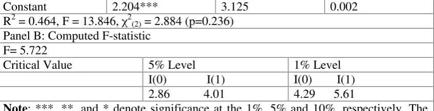
However, the unit root tests are performed to ensure that the order of integration of each variable does not exceed one. Table 1 shows the results of the Augmented Dickey-Fuller (ADF) and the Phillips and Perron (PP) tests.

Table 1Results of unit root tests Variable ADF test with

constant

ADF test with constant and trend

PP test with constant

PP test with constant and trend

Level

LM -0.883 (1) -2.548 (1) -1.067 (6) -3.852**(5) LRER -3.158** (1) -4.332*** (1) -2.814* (2) -3.957***(5) LY -1.355 (2) -2.882 (0) -1.291 (9) -2.892 (1) First difference

Δ LM -21.429***(0) -21.376***(0) -21.606***(1) -21.670***(1)

Δ ERE -9.574***(0) -10.037***(1) -9.368***(17) -9.362***(17)

Δ LY -11.703***(1) -11.771***(1) -13.139***(8) -13.151***(8)

Note: The number in parenthesis is the optimal lag. The optimal lag length of ADF tests is determined by Schwerz information criterion (SIC), and the optimal bandwidth of PP tests is determined by Bartlett kernel. ***, **, and * denotes significance at the 1%, 5% and 10%, respectively.

Therefore, it is likely that the three series are mixed between I(0) and I(1) and thus the use of bounds testing for cointegration should be suitable.

Results of Measuring Real Exchange Rate Uncertainty

The model of AR(p)-EGARCH(1,1) model expressed in equations (3) and (4) is estimated. The lag orderpof the mean equation is selected by SIC is 1. The estimated coefficient of log (ht-1) is 0.958 and is significant at the 1 percent level. However, the

estimated coefficient γ is -0.005 and is insignificant. Therefore, there are no

asymmetric impacts. Nevertheless, the results indicate the existence of persistence of shocks to conditional variance or real exchange rate volatility.

Table 2Result of AR(1)-EGARCH(1,1) model estimation Panel A. Mean equation:

Rt= 0.001 + 0.327***Rt-1+ εt

(0.621) (5.051)

Panel B. Conditional variance equation:

1 1

1 1

1 0.128 0.005 log

* * * 958 . 0 * * 492 . 0 log

 

 

  

 

t t t

t t

t

h h

h

h ε ε

(2.882) (59.283) (1.391) (-0.105) (t-statistic in parenthesis)

R2= 0.094, Log likelihood = 507.937

Q(4) = 4.724 (p=0.317), Q(8) = 4.938 (p=0.764) Q2(4) = 5.040 (p=0.283), Q2(8) = 10.228 (p=0.249)

Note: The number in parenthesis is t-statistic. *** denote significance at the 1% level.

The Box-Pierce Q(k) and Q2(k) statistics do not indicate any serial correlation and further ARCH effect at 4 and 8 lags (or k=4 and k=8). Therefore, a higher order of ARCH process is not required. In other words, the estimated model passes diagnostic tests. Furthermore, the GARCH variance or exchange rate uncertainty series is stationary.

Results of ARDL Model Estimates

The results of ARDL bounds testing for cointegration are reported in Table 3.

Table 3Results of ARDL bounds testing for cointegration.

Panel A: Estimated equation with Δ LMtas dependent variable

Variable Coefficient t-statistic p-value

Δ LMt-1 -0.385*** -5.408 0.000

Δ LRERt -0.057 -0.216 0.830

Δ LRERt-1 0.337 1.463 0.145

Δ LYt 0.532*** 5.863 0.000

Δ LYt-1 -0.183 -1.409 0.161

Δ LVt 13.932 0.118 0.698

LMt-1 -0.256*** -4.366 0.000

LRERt-1 -0.040 -0.388 0.698

LYt-1 0.245*** 3.650 0.000

Constant 2.204*** 3.125 0.002 R2= 0.464, F = 13.846, χ2(2)= 2.884 (p=0.236)

Panel B: Computed F-statistic F= 5.722

Critical Value 5% Level 1% Level I(0) I(1) I(0) I(1) 2.86 4.01 4.29 5.61

Note: ***, **, and * denote significance at the 1%, 5% and 10%, respectively. The critical values are from Table CI iii, Case III (unrestricted intercept and no trend) of Pesaran et al. (2001). The lower bound critical value is for I(0) series, and the upper bound critical value is for I(1) series.

The test results show that the restricted null hypothesis of the long-run coefficients (H₀:µ₁ µ₂ µ₃ µ₄ 0) is rejected at the 1 percent level of significance.8 This indicates that there is long-run relationship between imports and other variables (real effective exchange rate, real income, and real exchange rate uncertainty). The ARDL model passes diagnostic test because the Chi-square statistic [χ2(2)=2.884(p=0.236)]

indicates an acceptance of the null hypothesis of no autocorrelation in the residuals.

Results of Long-Run and Short-Run Estimates

The long-run relationship estimate is shown in Panel A of Table 4.

Table 4Results of long-run relationship and short-run dynamics Panel A. Long-run relationship: LMtis dependent variable

Variable Coefficient t-statistic p-value LRERt -0.269* -1.987 0.069

LYt 1.020*** 27.679 0.000

LVt -62.692*** -3.871 0.000

Constant 8.702*** 14.097 0.000 R2= 0.906, F = 537.766

Panel B. Short-run dynamics: Δ LMt is dependent variable

Variable Coefficient t-statistic p-value

Δ LMt-1 -3.079*** -5.412 0.000

Δ LRERt -0.187 -0.754 0.452

Δ LRERt-1 0.380* 1.704 0.090

Δ LYt 0.551*** 6.166 0.000

Δ LYt-1 -0.191 -1.536 0.127

Δ LVt 82.351 1.536 0.127

et-1 -0.257*** -4.486 0.000

Constant 0.006 1.156 0.249 R2= 0.455, F = 19.408

Note: ***, **, and * denote significance at the 1%, 5% and 10%, respectively.

8

The result shows that the estimated coefficient of real effective exchange rate is negative and significant at the 10 percent level while that of domestic real income is positive and significant at the 1 percent level. The two determinants of import demand have the opposite and correct signs as stipulated by the theory of international trade. The estimated coefficient of real effective exchange rate implies that a 1 percent increase in real exchange rate (or real depreciation) leads to a decline in real imports by 0.269 percent and vice versa. This result seems to support with the Marshall-Lerner condition, but with a weak support by the size of the coefficient and the 10 percent level of significance. For domestic real income, a 1 percent increase in real income induces an increase in real imports by 1.020 percent and vice versa. Similar to other developing countries, the impact of domestic real income is not surprising because Thailand relies on a high import portion of capital goods and raw materials in order to assist its export-led growth and import substitution strategies. The increasing importance of industrial sector has been observed since the 1990s. The negative impact of exchange rate uncertainty on real imports is large and significant at the 1 percent level. The result implies that an increase in this kind of uncertainty by 1 percent will significantly reduce real imports by almost 63 percent and thus improve

the country’s balance of trade, but can harm industrial sector at the same time.

The result of short-run dynamics is shown in Panel B of Table 4. The estimated coefficient of the error correction term (λ) is -0.257 and significant at the 1 percent level. This result indicates that the speed of adjustment to the long-run equilibrium is rapid. In other words, any deviation from the long-run equilibrium will be temporary. In addition, there seems to be no relationship between real effective exchange rate and import demand in the short run. Furthermore, there is a positive relationship between real imports and domestic real income. Also, exchange rate uncertainty does not impose any impact on real imports in the short run.

It should be noted that the presence of higher uncertainty in real effective exchange rate in the short run cannot induce a large number of manufacturing firms to increase or decrease their imports of capital equipment and raw materials so as to hedge against real depreciation in the near future. However, the effect of higher uncertainty in real effective exchange rate will induce most firms to delay their imports in the long run. In other words, importers will tend to import less when facing with higher real exchange rate uncertainty. The result from the present study seems to support the idea that importers are risk averse and substitute domestic for foreign goods (De Grauwe, 1988). In addition, importers will reduce imports when they encounter unpredictable exchange rates, which cause uncertain profits (see Gotur, 1985, among others).

CONCLUDING REMARKS

dynamics shows that the coefficient of the error correction term is significantly negative and has the absolute value of less than one, which implies that any deviation from the long-run equilibrium will be corrected rapidly. The findings obtained from this study give some implications for policymakers. First, an appreciation of real effective exchange rate will induce more imports and lead to deterioration of balance of trade in the long run, and vice versa. Second, an increase in real sector production will induce more imports and vice versa. Third, stabilization of major nominal exchange rates to reduce exchange rate uncertainty and the design of appropriate trade policy seem to be necessary.

REFERENCES

Akpolodje, G., and Omjimite, B. U. (2009) “The effect of exchange rate volatility on the imports of ECOWAS countries” Social Sciences, Vol. 4, pp. 304-346.

Alam, S. (2012) “A reassessment of Pakistan”s aggregate import demand function: An application of ARDL approach” Journal of Developing Areas, Vol. 46, 367-384.

Arize, C. A. (1998) “The effects of exchange rate volatility on US imports: An empirical investigation” InternationalEconomic Journal, Vol. 12, pp. 31-40.

Arize, C. A., Osang, T., and Slottje, D. J. (2008) “Exchange-rate volatility in Latin

America and its impact on foreign trade” International Review of Economics and

Finance, Vol. 17, pp. 33-44.

Arize, C. A., and Walker, J. (1992) “A reexamination of aggregate import demand in

Japan: An application of Engle and Granger two-step procedure” International

Economic Journal, Vol. 26, pp. 41-55.

Bollerslev, T. (1986) “Generalized autoregressive conditional heteroskedasticity”

Journal of Econometrics, Vol. 31, pp. 307-327.

Caporale, T., and Doroodian, K. (1994) “Exchange rate variability and the flow of international trade” Economics Letter, Vol. 46, pp. 49-54.

Coric, B., and Pugh, G. (2010) “The effect of exchange rate variability on international trade: A meta-regression analysis” Applied Economics, Vol. 42, pp.

2631- 2644.

De Grauwe, P. (1988) “Exchange rate variability and the slowdown in the growth of international trade” IMF Staff Papers, Vol. 35, pp. 63-84.

Doroodian, K. (1999) “Does exchange rate volatility deters international trade in developing countries?” Journal of Asian Economics, Vol. 10, pp. 465-474.

Erdem, E., Nazlioglu, S., and Erdem, C. (2010) “Exchange rate uncertainty and

agricultural trade: Panel cointegration analysis for Turkey” Agricultural Economics,

Gotur, P. (1985) “Effects of exchange rate volatility on trade” IMF Staff Papers, Vol.

32, pp. 475-512.

Hassan, S., and Wallace, M. (1996) “Real exchange rate volatility and exchange rate

regimes: Evidence from long-term data” Economics Letters, Vol. 52, pp. 67-73.

Hegerty, S. W., Harvey, H., and Bahmani-Oskooee, M. (forthcoming) “Empirical

tests of the Marshall-Lerner Condition: A literature review” Journal of Economic

Studies, Vol. 40.

Himarios, D. (1989) “Do devaluations improve trade balance? Evidence revisited”

Economic Inquiry, Vol. 27, pp. 143-168.

Hooper, P., and Kohlhagen, S. (1978) “The effect ofexchange rate uncertainty on the

prices and volume of interntional trade” Journal of International Economics, Vol. 8,

pp. 483-551.

Kenan, P., and Rodrik, D. (1986) “Measuring and analyzing the effects of short-term

volatility in real exchange rate” Review of Economics and Statistics, Vol. 68, pp. 311-315.

Miles, M. A. (1979) “The effects of devaluation on the trade balance and the balance of payments: Some new results” Journal of Political Economy, Vol. 83, pp. 600-620.

Naseem, N. A. M., Tan, H-B., and Hamizah, M. S. (2009) “Exchange rate misalignment, volatility and import flows in Malaysis” International Journal of

Economics and Management, Vol. 3, pp. 130-150.

Nelson, D. (1991) “Conditional heteroskedasticity in asset returns: A new approach”

Econometrica, Vol. 59, pp. 347-370.

Pesaran, M., Shin, Y., and Smith, R. (2001) “Bounds testing approaches to the analysis of level relationships” Journal of Applied Econometrics, Vol. 16, pp. 289 -326.

Siregar, R., and Rajan, R. S. (2004) “Impact of exchange rate volatility on Indonesia’s trade performance in the 1990s” Journal of the Japanese and International Economies,

Vol. 18, pp. 218-240.

Tang, T. C. (2004) “A reassessment of aggregate import demand function in the

ASEAN-5: A cointegration analysis” International Trade Journal, Vol. 18, pp. 239-268.

Warner, D., and Kreinin, M. E. (1983) “Determinants of international trade flows”

Review of Economics and Statistics, Vol. 65, pp. 96-104.

Zhang, Y., Chang, H., and Gauger, J. (2006) “The threshold effect of exchange rate volatility on trade volume: Evidence from G-7 countries” International Economic