Finite Difference Preconditioners for Legendre Based
Spectral Element Methods on Elliptic
Boundary Value Problems
*
Seonhee Kim1, Amik St-Cyr2, Sang Dong Kim1#
1Department of Mathematics, Kyungpook National University, Daegu, South Korea 2Computation and Modeling, Shell Technology Center Houston (STCH), Houston, USA
Email: [email protected], [email protected], #[email protected]
Received November 13,2012; revised April 1, 2013; accepted April 8, 2013
Copyright © 2013 Seonhee Kim et al. This is an open access article distributed under the Creative Commons Attribution License, which permits unrestricted use, distribution, and reproduction in any medium, provided the original work is properly cited.
ABSTRACT
Finite difference type preconditioners for spectral element discretizations based on Legendre-Gauss-Lobatto points are analyzed. The latter is employed for the approximation of uniformly elliptic partial differential problems. In this work, it is shown that the condition number of the resulting preconditioned system is bounded independently of both of the polynomial degrees used in the spectral element method and the element sizes. Several numerical tests verify the h-p independence of the proposed preconditioning.
Keywords: Finite Difference Preconditioner; Iterative Method; Spectral Element Method; Elliptic Operator
1. Introduction
Linear systems engendered by spectral element discreti-zations of a simple second-order elliptic boundary value problem have large condition numbers depending on the number of elements E and the polynomial degree N em-ployed. Convergence of iterative solvers thus deteriorates as E and N increases. Regardless of these restrictions, the spectral element method is very popular, accurate and used in many engineering problems. However, it is widely known that an efficient preconditioner is neces-sary in order to improve the convergence of Krylov sub-space methods traditionally used to solve the resulting linear system (see [1-7]). Since the work of [8], it is nu-merically known that finite difference preconditioning of the spectral element matrix leads to satisfactory results in terms of convergence rates. Multigrid methods are opti-mal in terms of convergence rate and have linear cost for finite difference problems. The Algebraic multigrid (=: AMG) method can be easily applied to finite difference discretizations of elliptic operators. If it is instead applied directly to high-order discretizations, such as spectral ele-
ments, some outstanding issues still need to be addressed. The idea of employing a low-order discretization com-bined with multigrid as the preconditioner of a high-or-der problem was investigated in [9] where P1 finite
ele-ments were employed instead of finite differences. Other efforts concerning the computational cost of P1 finite
element based two levels additive Schwarz precondition-ers can be found in [10,11]. In both approaches an inter-mediate problem for the Laplace equation was con-structed using the high-order Legendre-Gauss-Lobatto (=: LGL) nodes. Furthermore, analytic work was performed in [12] for a second-order uniformly elliptic boundary value problem using LGL nodes and also the analytic research based on Chebyshev-Gauss-Lobatto (=: CGL) nodes was done in [13], in which the various node con-figurations (LGL and CGL nodes) were employed for the construction of the P1 finite element preconditioner. In
the 1- and 2-dimensional case, the approach was proven optimal and scalable, respectively.
Thus an efficient and optimal algorithm, with linear cost, for solving problems based on spectral element dis-cretizations, which guarantees the convergence of the overall preconditioning strategy, is readily available. The P1 finite element matrix lowers the complexity of the
system to invert since the matrices, representing the Laplacian, are tri, penta or hepta diagonal and are easily solvable using the multigrid method.
*The third author (corresponding) was supported by basic science re-search program through the National Rere-search Foundation of Korea (NRF) funded by the ministry of education, science and technology (grant number 2010-0008317) and Kyungpook National University Research Fund 2012.
Recently Canuto et al. [14,15] have discussed precon-ditioning with low order finite-elements methods. They show the equivalence between spectral elements and low order finite-elements. The proof is shown for finite-ele- ments and so called numerical integration (NI). In our approach, following motivations found in [4], we pro-pose another preconditioning approach using a simple finite difference scheme based on the LGL nodes in a pointwise approximation perspective. The latter is repsented as tensor product matrices, and finite element re-lated properties are employed to prove its optimality. Additionally, it is shown that the proposed precondition-ers herein are optimal from the theoretical analysis standpoint and that optimality is confirmed with numeri-cal experiments.
The paper is organized as follows. First, the problem is described in Section 2 and basic definitions are recalled in the same Section 2 also. In the same section, the finite difference preconditioner is introduced. In Section 3, a uniform bound for , the ratio of LGL weights to the distance between the adjacent LGL nodes, is derived which will be used for the 2D case. The optimality re-sults are presented in Sections 4 and 5 with the numerical experiments which support the developed theories. Fi-nally, conclusions are drawn.
q
2. Description of the Problem
Consider the classical boundary value problem of a sec-ond-order elliptic operator
: in n,
Au p u qu n1, 2, (2.1) where 1
pC and qC
are satisfying0 1 1
0p p p , 0 q q . (2.2) The resulting matrix for the operator A, with variable coefficients, discretized using spectral element methods based on LGL nodes is represented as AˆhN and 2 2
h N
in one- and two-dimensional case, respectively. Two- dimensional matrix 2 2
h N is the result of tensor
prod-ucts using the matrices obtained in the one-dimensional case. We shall consider the preconditioner h
ˆ A
ˆ A
ˆ
A and 2
h
ˆ A for the 1D and 2D case, respectively. Then the problem is to demonstrate the validity of the preconditioners for
ˆ
h
L
ˆ
hN
A and 2
h for h N2 2, respectively. Moreover,
the goal is to show that the preconditioners are optimal in the sense that the condition numbers of the precondi-tioned systems hN and 2 2 2
h h N for each case are
independent of mesh sizes ˆ
L
1
ˆ
h
L A ˆ A
ˆ 1ˆ
L Aˆ
j
h of elements and degrees
k of the piecewise polynomials employed in spectral
element discretization. N
For the above goal, we will introduce some notations and definitions from now on. Let
N0 and
k 0k k
N
k
be the reference LGL points in
1,1
and quadrature weights associated with the -degree Legendrepoly-nomial. With dimensionless notations t, let us denote
th
N
E0 j jt
as the knots in the interval I
1,1
such that0 1 E 1 E: 1.
t t t t
1 :
For convenience, we de- note Nj as the degree of Legendre polynomial on each
subinterval Ij: tj1,tj . k will be the sum of
the degrees of each element up to k:
1 N
k j
j . In
par-ticular, the notation
N
: NE
N is used when k = E
and
N0 0. The translated LGL points and corre-sponding weights from
N0 and
arek k
0
N k k
1
, ,
1, 0
: j
j
E N j k k N
j k
with
, 1
1 ,
2 2
j
1
j k k j
h
t tj hj tj tj (2.3)
and, respectively,
,0
j
N j k k
:
, :
j k
1 0
1, 1, 2,
,
2 2
1, 2,
j j
j k
, 2
j
j k
N
h
N
h h
0 or , , 1,
, 1,
j E
j E
, 2, ,
,
E j
j
j E k N
k
k N
1
1,0
(2.4)
and j :j N j, for j1, 2, ,E1
0 N
: 1
.
For simplicity, all LGL points are arranged as 1 :01N
j k,and the corresponding LGL weights are ordered as ,
1, 0 :
j E N
j k
0
N
with
1,0:
E tE
. Notice that from (2.3) j N, j j1,0 for
1, 2,
j ,E1
k
follows.
Let be the space of all polynomials pk
t de-fined on
1,1
h
I whose degrees are less than or equal to k and let N be the subspace of , which
con-sists of piecewise polynomials
j
N with support
1
C I
p t
,
j j j
I t t whose degrees are less than or equal to
j
N . Let N be the space of all piecewise Lagrange
linear functions ˆk
t with respect to 0k
kN
on
1,
I 1 . Define h N
as the space of all Lagrange piecewise linear functions with respect to .
Let
t
1 0
H I
H
be the standard Sobolev space with zero boundary conditions. Let 0 :H1h and
, 0
h N N
be the finite dimensional subspaces of
0 , :
h N
1h
0 N
1 0
H I with the basis functions
and
1d
1
d
respectively, where h N, h N, . To
communicate between the space of piecewise linear functions and the space of piecewise polynomial, we use the interpolation operator such that
0 dim
I
0: dim
:
h N C I
d
h N
Nhv
v for vC I
.ordered by horizontal lines or, more precisely, all the
points are listed as
,1: , 1, 1
x y
xy d d
d
, where
1x
d
for 1, 2, , dx, 1, 2, , dy. Forthe two-dimensional high-order and piecewise linear space, let
2
0 0 0
, : x, x y, y,
h N h N h N
and
2
0 0 0
, : x, x y, y
h N h N h N
whose basis functions are given by tensor products of one-dimensional piecewise Lagrange polynomials and linear functions, respectively. Let
0 2
,
: dim
xy
h N
d . Note that xy x y
t x
d d d , where
,,
: dim t t t
h N
d 0
or y.
To provide the preconditioner, using the global LGL points
, we define the operator Bh on0 ,
h N
11 1
1 1
,
h
u u
B u u
s s s s
1 (2.5)
where s:1, u:u
.With this operator and components 0, 0, we define the one-dimensional finite difference operator
as following: h
L
L uh
B uh s u ,where s:ss111
The two-dimensional finite difference operator is therefore defined as
.
2 h
L
2 , , ,
,
, ,
y x x
h h
x y y
h
L u s B u s u
s B u s u
(2.6)
where
,
t h
B u
is the 2D version of (2.5) for tx or y, precisely,
1, 1,
, ,
1 1
, 1 , 1
, ,
1 1
1 1
: ,
1 1
: ,
x
h x x x x
y
h y y y y
u
B u u
s s s s
u u
B u u
s s s s
u
(2.7)
and st t1t, stt1t1 for tx or y and
: ,
u , u .
Finally, the notation for any two real quantities a and b is a shorthand notation corresponding to the ex-istence of two positive constants c and C, which do not
depend on the mesh sizes and the degrees of polynomials
ab
such that 0 c a C
b .
The notation (U, V) stands for
u vi i for any two vectors andd where the superscript T denotes the
transpose of a vector or matrix. The standard Sobolev space H1 and L2 will be used. And we will use
T1, , d
U u u
1, ,V v v
T1
, 1
and 0 as the standard Sobolev H1-norm, H1-seminorm
and the usual L2-norm, respectively.
3. Basic Estimates
We begin by recalling the relations between the distances of LGL nodes and the LGL weights in the reference element
1,1
found in [6].Lemma 3.1. With LGL nodes k and LGL weights
k
, let
0 0
1 0 1
2 2
: , : N
N
N N
q q
,
(3.1)
1 1
2
: k , 1, ,
k
k k
q k
1.
N
N
(3.2)
Then the qk are uniformly bounded for all
0,1, ,
k . In particular,
1 0 2 1 2
0 q and 0 qN , (3.3)
where i, 1, 2i
i
are constants independent of thepolynomial degree N.
Proof. See Lemma 3.1 in [6]. □ Since the goal is to develop preconditioners on spec-tral elements considering different polynomial degrees on each elements of which sizes are not identical, we need an advanced version or -version of Lemma 3.1. Hence the modifications of (3.1)-(3.2) for
,, 0: 1, 0
j E N
j k j k
q q
N are required, where
j1k N
0
q .
First, let , qN and q be
defined as
1, 2, , 1
N
0 0
1 0 1
2 2
: , :
q q
N
N
N N
, (3.4)
and
1 1
2
: for 1, 2, ,
q
1.
N (3.5)
Lemma 3.2. The q given in (3.4)-(3.5) are bounded for all 0,1, , N independently of both degrees k
of polynomials and the mesh sizes
N
j
1,0 0 1,1 1,0
,
, , 1
, ,
, 1 , 1
,
, , 1 1,1 1,0
2
,
1, 0, 2
,
, ,
2 ,
1, 2, , , 1, 2, , 1, 2
,
1, 2, , 1, .
E
E E
j
j j
E N E N E N
E j k
j k j k j k
j j N
j N j N j j
j
q
j k
q
j E k N
q q
j E k N
j E k N
N
(3.6) Since the first and second cases of (3.6) are
1 0
0 0
1 1 0
2 2
2 h
q q
h
and
1
2
2 ,
2
E
E
E E
E N
N E
N N
h
q q
h
N
it is clear that , are uniformly bounded by Lemma 3.1. 0
q qN
For the case , , it can
be easily shown that 1, 2, ,
j E k1, 2, , Nj1
, ,
, 1 , 1
1 1
2
2 2
. 2
j k j k
j k
j
j k j k
k k
h
q
h
qk
Lastly for j1, 2, , E1, kNj, note that
1
1 0 ,
1 1 0 2
2 2
.
2 2
j
j
j j
j j
N j N
j j
N N
h h
q
h h
1 Using (3.3), it comes
1 0
10
1 0
and
NjNj1
2 Nj
Nj Nj1
2,where are the absolute positive constants that appear in Lemma 3.1. Therefore,
, 1, 2
i i i
1 2
,
1 22 min , qj Nj 2 max ,
which completes the proof. □ Define the two matrices W and H, which are made up of, respectively, the quadrature weights and the distances between the LGL points:
1 1
1 : diag , : diag
diag diag ,
W
H
s s s
(3.7)
where 1, 2, , d and 0d10.
Notice that the quantities 11 and are positive for all 1, 2, , d. By Lemma 3.2, q de- fined in (3.5) are uniformly bounded. Thus we have the following corollary:
Corollary 3.3. For U
u u1, , ,2 ud
T, it follows that
HU U,
WU U,
.The next result is a clear consequence but we write down for convenience.
Lemma 3.4. For any diagonal matrix S with
nonnega-tive entries whose size is the same as W (see definition in (3.7)),
SW U U,
WU U,
,where the equivalence depends on the minimum and maximum entries of S.
The matrix W will be replaced by for two- dimensional problems.
WW
Proposition 3.5. Let be symmetric and positive definite matrices such that
,
E F
EV V,
FV V,
(3.8)for any nonzero vector . Then for any symmetric and positive definite matrix , we have
V G
, ,
, ,
G E V V G F V V
E G V V F G V V
,
. (3.9)
Proof. Since all the matrices are symmetric and posi-tive definite, it is enough to discuss (3.9) in terms of ei-genvalues.
Consider the eigenvalue problem
.
EU FU
It has a complete set of eigenpairs
U,
, 1, 2, , xd
. Let
, 1
Z 1U , (3.10) where 1 is a vector consisting of element 1 with length
y
d .
= 1
,
G E Z G E U G EU
G FU G FU
G F U
G F U
G F Z
1 1
1 1
1
1
the vectors and eigenvalues in (3.10) are complete sets of eigenvectors and eigenvalues of the eigenvalue problem
GE V
GF V
.From (3.8), since are positive, bounded and inde- pendent of x
j
h , Nkx, so are . Therefore it follows
GE V V,
GF V V
,
for any vector .V By the same reasoning, it follows
EG V V,
FG V V
,
. □Finally, the known results stated in Theorem 3.3 and 3.5 from [12] are recalled here for completeness.
Theorem 3.6. It follows that for all uNh,
1 0
1 and 0 .
h h
Nu u Nu u
4. One-Dimensional Case
Before going ahead, suppose that 1
pC and
qC satisfy 0 pˆl p x
pˆu u pˆl pˆu qˆl
and , where , , and are constants. Now consider the following elliptic boundary value problem with zero boundary condition:
ˆ ˆ
0ql q x q qˆu
:
Au p x u x q x u x in 1,1 . (4.1) Expanding and in (4.1) on the space
as
1p x
d
q x
0 ,
h N
p x
p and q x
d1q , the matrix representation of the operator A in (4.1) by the spectral element discretization based on LGL points is now given by
T
ˆ :hN ,
A D PW D QW (4.2)
where , , D is
the differentiation matrix defined as
1
diag , , d
P p p Qdiag
q1, , qd
:
D and W is the matrix defined in (3.7).
Since P and Q are the diagonal matrices with non-negative elements, by Lemma 3.4 we have for any vector U,
KU U ,
:
DT
PW D U U
,
D WD U UT
,
and
QWU U,
WU U,
.More precisely, it follows that
T
T
ˆl , , ˆu ,
p D WD U U KU U p D WD U U ,(4.3)
ˆl , , ˆu
q WU U QWU U q WU U,
. (4.4) Besides, we can see that for
0, 1
d
N h N
u t
u t ,
2 T
1
2 0
, ,
, ,
N
N
D WD U U u
WU U u
(4.5)
where U
u u1, , ,2 ud
T.ˆ
h
B
Let be the matrix representation of , which is
defined in (2.5). For , the easy
calculation leads to
h
B 0 ,
h N
1
d
u t
u t
2
0 1 ˆh ,
C u B U U C u1 21, (4.6) where U
u u1, , ,2 ud
T.Note that the constants such as 0, 1 appeared in
this and next sections are generic positive constants, in-dependent of the number of elements i and the degree
C
E C
j
N of polynomials applied to spectral discretization. Now to provide a finite difference type preconditioner, consider the bilinear form with a positive constant
0
,
N
l u v
, defined on the space 0 0
, h N,
h N
d
0
1, ,
N h
l u v B u v
where u u
0
. This induces the matrix Lˆh,0:
,0 ˆ
, ,
N h
l u v L U V ,
.ˆ
h
T
T1, , d , , ,1 d
U u u V v v
Thus it comes immediately
,0
ˆ .
h
L B (4.7)
Lemma 4.1. For any vector , it
follows that
T1, , ,2 d
U u u u
0 1
,0
ˆ , max ˆ ˆ,
ˆ
0 .
ˆ ,
hN u u
l h
A U U p q
p
C C
L U U
Proof. Note that 0 can be expressed as
,
h N
u
t
1
d
u t
u , so that its piecewise polynomial interpolation becomes
0, 1
d h
Nu t
u t h N .
Since
KU U ,
A U UˆhN ,
KU U ,
QWU U,
, it follows from (4.3)-(4.5), that
2 2
1 1
2 1
ˆ
ˆ , max ˆ ˆ,
ˆ ˆ
max , .
h h
l N hN u u N
h u u N
p u A U U c p q u
C p q u
Therefore, (4.7), (4.6) and Theorem 3.6 complete the proof. □
Remark 1. From the above lemma, one may notice
that the upper bound for the condition numbers of the matrix does not depend on the mesh size hj of
an element and the degree Ni of a polynomial. Further, it
does not depend on
1 ,0ˆ
ˆ
h hN
L A
. Hence, even if (4.1) has coeffi-cient functions p x
and q x
ˆ B
, it is enough to take the preconditioner Lˆh,0 h with 1 in (4.7).
Next, we consider another bilinear form lN
u v, on the space 0 0 with a constant, ,
h N h N
0
0
1
, : , d ,
N N
l u v l u v s u v
where uu
and s11
,N
l
. The matrix representation Lˆh corresponding to
is
,
ˆ ,
N h
l u v L U V ,
.
T
T1, , d , , ,1 d ,
U u u V v v
where
ˆ : ˆ
h h
L B H (4.8) Now the goal is to analyze the validity of the matrix operator Lˆh for the preconditioner to AˆhN.
Theorem 4.2. For any vector , it
follows that
T1, , ,u2 ud
U u
ˆ ,
ˆ ,
hN h ,
A U U L U U
where the equivalence depends only on , , , ,
ˆu
p pˆl qˆu
ˆl
q and .
Proof. For such that ,
its piecewise polynomial interpolation is
0 ,
h N
u u t
1
td
u
0, 1
d h
Nu t
u t h N
. Using (4.3)-(4.5), we get
2 ˆ
ˆ ˆ h
1
2 1
min , ,
ˆ ˆ
max , .
l l N hN
h u u N
c p q u A U U
C p q u
On the other hand, applying Corollary 3.3, (4.5) and Theorem 3.6 we have
2 0, 0
, for h N
HU U u u (4.9)
so that
2
21 ˆ 1
min , h , max ,
c u L U U C u .
Hence, using Theorem 3.6 again, we have
0 1
ˆ ,
ˆ ˆ ˆ
min , max ,
. ˆ
max , , min ,
hN
l l u u
h
A U U
p q p q
C C
L U U
ˆ
To guarantee the positivity of the lower bound, if , we will take
ˆl 0
q 0. Applying Poincare’s
ine-quality with (4.9) and (4.6), we have
,
ˆ
h ,
HU U C B U U for some positive constant C. Therefore, using (4.3)-(4.5) and Theorem 3.6, we get
1
, , ,
ˆ ˆ ˆ max u, u h ,
KU U QWU U
C p q B U
0ˆl ˆh
c p B U U
U
so that
0 1
ˆ , max ˆ ˆ,
ˆ
, ˆ ,
hN u u
l h
A U U p q
p
C C
L U U
which leads to the conclusion.
The latter, combined with the min-max theorem, yields the next result.
Corollary 4.3. The eigenvalues
1d
of
are all positive real and bounded above and below. The bounds are independent of the mesh sizes hj and the
degrees of the polynomials Nk. That is, there are absolute
constants and such that
1ˆ
ˆ
h hN
L A
0
C C1
0 1
0C C .
Remark 2. Theorem 4.2 reveals that the condition
numbers of L Aˆh1ˆhN are bounded above by
ˆ ˆ
max , ,
ˆ ˆ
min , min ,
u u
l l
p q p q
max
or max
ˆ ˆ,
ˆu u l
p q
p . Hence one
may notice that the condition numbers do not depend on the degrees of polynomials Nk and the mesh sizes h . j
According to Remark 2, we may summarize the be-havior of the condition numbers of in the fol-lowing corollary.
1ˆ
ˆ
h hN
L A
Corollary 4.4. The upper bound of the the condition
numbers of L Aˆh1ˆhN behaves like
ˆ
ˆ
u l
p p ,
ˆ ˆ
u l
q p ,
ˆ ˆ
u l
p q or ˆ
ˆ
u l
q q .
We will investigate the efficiency of the precondition-ers Lˆh,0Bˆh and Lˆh BˆhH for several
prob-lems with constant and variable coefficients. Moreover, for a variable coefficients problem, we will compare the developed preconditioners with the 1 finite element
preconditioner (see [12]) in terms of iteration numbers using the preconditioned conjugate gradient method (=: PCG).
P
Example 1. Consider the operator with constant coef-ficients:
: in
Au puqu 1,1
(4.10) with homogeneous Dirichlet boundary conditions, where and are constants. Note that the spectral element discretized matrix corresponding to (4.2) be-comes0
p q0
T ˆ
hN
definition, we take 1 and focus mainly on the role of , where Lˆh BˆhH.
First, it is computed with ,0 h. Figure 1 is
shown to be ineffective for large values ˆ
h
L Bˆ
q p, but we can see that Lˆh,0Bˆh is effective for q p-value equal
or less than 1 (see Table 1).
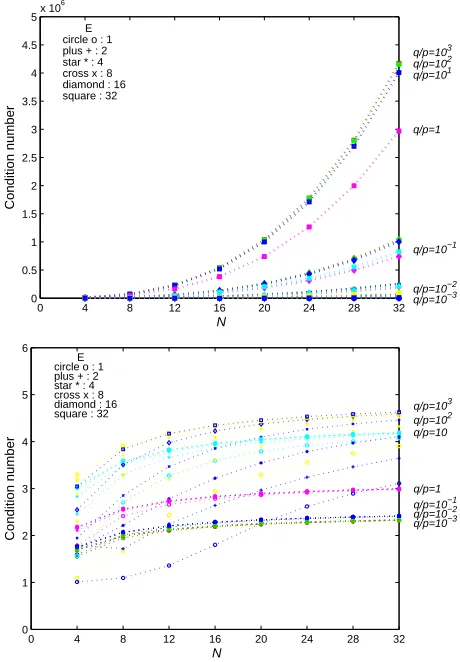
Second, to show that the preconditioning work is not independent of the polynomial degrees N and the num-bers of element E, applied in spectral element method, it is tested for the cases with N4,8,12, ,32 and
. For the values 1,
2, 4, ,
E 32 q p10 ,10 , ,103 2 T
3,
the condition numbers of AˆhN pD WDqW
32 N E
ˆ ˆ
h h
L B
go up to
approximately when , but ones of
the matrices preconditioned by ,0 are bounded
[image:7.595.308.538.86.417.2]above by approximately 4.5, independently of N, E (see
Figure 2).
6
10
4.5
Third, We investigated the condition numbers of the matrices by preconditioned by LˆhBˆhH with sev-
eral -values for each q p-value (see Figure 3). When is taken to be equal to q p-value or
1,q p
,preconditioning results (see Figure 4).
Example
max it give
with h
ˆ q
s good
2. No onsider the operator with the va
1,1 (4.11)
omogeneou undary
w we c
pu s Dirichlet bo
are constants. In this riable coefficients:
: in
Au qu
conditions, where
ˆ
2 1
p x p x and q x
qˆ cosx , where ˆ 0p the spectra ment discretization yield the matrix
T
ˆ ˆ ˆ
hN
and 0 case, l
ele-A pD PW DqQW , where P and Q are the ma es of 2 1
x o
tric and c sx represented b spectral y
10−5 10−4 10−3 10−2 10−1 100 101 102 103 104 105
0 0.5 1 1.5 2 2.5 3 3.5
4x 10
4
q/p
Condition number
Figure 1. Condition numbers of where
1. Condition numbers of where ˆ
ˆ
h hN
L A1 ,0
, Lˆh,0Βˆh.
Table L Aˆh1,0ˆhN
, Lˆh,0Βˆh.
q p 105 104 103 102 101 10 0
0 4 8 12 16 20 24 28 32
0 0.5 1 1.5 2 2.5 3 3.5 4 4.5
5x 10
6
E circle o : 1 plus + : 2 star * : 4 cross x : 8 diamond : 16 square : 32
q/p=103 q/p=102 q/p=101
q/p=1
q/p=10−
Condition number
1
q/p=10−2
q/p=10−3 N
0 4 8 12 16 20 24 28 32
0 1 2 3 4 5 6
N
Condition number
E circle o : 1 plus + : 2 star * : 4 cross x : 8 diamond : 16
square : 32 q/p=10
3
q/p=102 q/p=10
q/p=1 q/p=10−1 q/p=10−2 q/p=10−3
Figure 2. Condition numbers of AˆhN and L Aˆh ˆhN where
1 ,0
, ˆ ˆ
h h
L,0Β .
10−5 10−4 10−3 10−2 10−1 100 101 102 103 104 105
0 0.5 1 1.5 2 2.5 3 3.5
4x 10
4
q/p
Condition number
β=104
β=103
ˆ ˆ
h hN
L A1
[image:7.595.307.537.369.645.2] ,
Figure 3. Behaviors of where LˆhΒˆhH.
element discretization, respectively. Figure 5 shows that
ˆ 2ˆ
q p
or max 1,
qˆ 2pˆ
give the good precon-ditioning esults.
Example 3. Fo oefficients problem of Example 2 with
r
r the variable c
2:3239 2:3238 2:3237 2:3236 2:3230 5:0419
2 1 [image:7.595.58.287.472.727.2]10−5 100 105 1010 1015 1.5
2 2.5 3 3.5 4 4.5 5
q/p
Condition number ← β = q/p
[image:8.595.58.285.87.262.2]↓
Figure 4. Condition numbers of , where
β = max(1,q/p)
ˆ ˆ
h hN
L A1 ˆ ˆ
h h
L Β βH.
10−5 100 105 1010 1015
1 2 3 4 5 6 7 8
q
1 / p1
Condition number
↑ β = q
1/2p1
← β = max(1, q1/2p1)
Figure 5. Condition numbers of L Aˆh ˆhN where
1
, LˆhΒˆh
βH.
1,1 ,
h
: in
Au puqu (4.12) we compute the iteration number using PCG precondi- tioned by LˆhBˆ . Also we compare the developed
preconditioners with the 1 finite element precon-
ditioner
ˆ
h
L
h
P
ˆ
F (see [10,12] for example) in terms of itera- tion numbers using PCG.
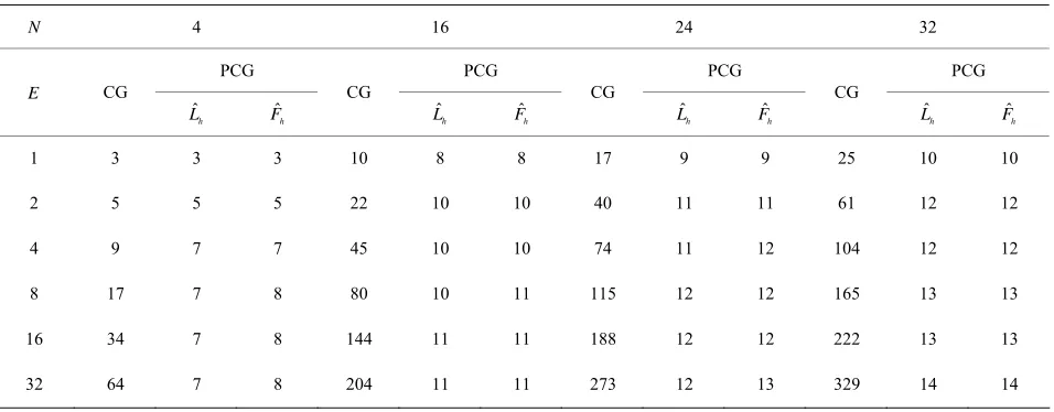
The computational results are shown in Table 2 with
various numbers of elements E and polynomial degrees N. While the number of iterations increases as N or E becomes large in case of CG iterations, the PCG precon- ditioned by gives relatively small. In particular, it can be predicted that the preconditioning effects become stronger as N or E are made larger. Furthermore we note that the results are comparable to the ones for finite element preconditioner.
ˆ
h
L
5. Two-Dimensional Case
In this section the tensor notation is employed. It has the
form y x
A B and the superscripts denote the spatial dimension on which it acts. Their order will always be the same and thus we omit them. For the tensor product representation, we refer to [16].
Consider the elliptic operator corresponding to 2D case with zero boundary conditions:
: , , ,
in 1,1 1,1 ,
, Au p x y u x y q x y u x y
(5.1)
where 1
pC and qC
are satisfying
ˆ ˆ
0pl p x y, pu , 0qˆl q x y
, qˆu .As in the 1D case, by expanding the variable co- efficients p x y
, and q x y
, in terms of the basis
dxy1
of
2 0 ,
h N
, two coefficients matrices are ob-
[image:8.595.56.288.94.501.2]tained:
Table 2. Iteration numbers in 1D.
N 4 16 24 32
PCG PCG PCG PCG CG
ˆ
h
L Fˆh
CG ˆ
h
L Fˆh
CG ˆ
h
L Fˆh
CG ˆ
h
L Fˆh
E
1 3 3 3 10 8 8 17 9 9 25 10 10
2 5 5 5 22 10 10 40 11 11 61 12 12
4 9 7 7 45 10 10 74 11 12 104 12 12
8 17 7 8 80 10 11 115 12 12 165 13 13
16 34 7 8 144 11 11 188 12 12 222 13 13
32 64 7 8 204 11 11 273 12 13 329 14 14
[image:8.595.61.539.547.734.2]
: d He the enval of
and bou ed. boun ar ent of the
iag ,
P p: p
: diag : ,
Q q q
1 .
x
d
Then the matrix from the spectral element discretiza-tion, using one-dimensional matrices and W, becomes D
T T
T ,
2 2
T
ˆ :
h N
A I D P W W I D
I M Q W W I M
D I P W W D I
M I Q W W M I
(5.2)
where
M is the 1D mass matrix, which becomes the
identity for the Lagrange basis
1
dxy
.
From the similar argument in 1 (4.4), we have
D case such as (4.3)-
p Wˆl K q Wˆ W
2 2
ˆ ˆ ,
ˆ , ˆ ˆ
ˆ ˆ ,
l
l l
u u
h N
u u
p K W q W W V V
A V V p W K q W W
p K W q W W V V
for any nonzero vector
In order to describe the preconditioner for the defined in (2.6), we c si
V .
2D on- case, with the operator
h
L2
der a bilinear form 2
,N
l on h N0, h N0,
2 , 2
d d
N h
l u v L u ,
, 1 1
: v ,
x y
which becomes
,
2 , ˆ2 ,
N h
l u v L U V where
2
ˆ : ˆ
ˆ
y x y x
h h
y x y
h
L H B H H
B H H H
x (5.3)
and ˆt is the matrix induced from (2.7) fo
h
B r each tx
or
tha
,
y.
Notice that in the proof of Lemma 4.1 it is shown t
,
ˆ
h
KU U B U U thi
is for any nonzero vector . Using
Theorem 5.1. Fo
U s fact and Proposition 3.5, we have the following:
r any vector V
v1, , v
T, we havexy d
Aˆh N2 2V V,
L Vˆh2 ,V
,where the equivalence are dependent o ly on n pˆu, pˆl,
ˆu
q , qˆl,
nce, nd
eig The
ues ds
2
h h2 2
1ˆ
ˆ
N
L A e independ
are all positive mesh sizes t
j
h and the degrees Nkt, where tx or .
Re ar 3. Thi res
y e,
k s ult cas that
th ion numb
m reveals, as in 1D
e upper bound for the condit ers of the matrix
2 2 2
1ˆ ˆ
h h N
L A is dependent only on the variable coefficients
,p x y and q x y
, , precisely the condition numbers are bounded above by
and .
ˆ ˆ max , max
ˆ ˆ
min , min ,
u u
l l
p q
p q
,
or
ˆ ˆu,qu
.
max ˆ
p
p
mple, the various eigenv d condition numbers of the preconditioned matrix are re-ported. They are compared with their finite element sibling. Also included is a comp iteration co
en
l
In the following exa alues an
1
P arison of the unts, for a PCG solver, for the proposed precondition-ers.
Example 1. Consider the homog eous Dirichlet boundary value problem
: in 1,1 1,1 ,
Au p u qu where p x y
, x y2 2x2y21 and
, cos cosq x y x y.
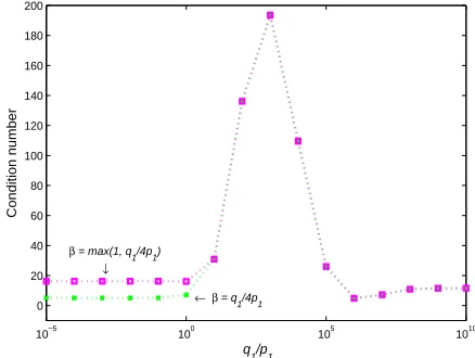
As in 1D case, we consider qˆ 4pˆ or
ˆ ˆ
max 1,q 4p to have a good preconditioning ork, re shown in Figure 6.
Example 2. For t homogeneous Dirichlet boundary va
w which a
he lue problem
:
Au u 10 inu 1,1 1,1 , we now compare the developed preconditioners w
2
h
ith the P1 finite element preconditioner ˆ2
h
ˆ L F in terms of iteration numbers using the PCG.
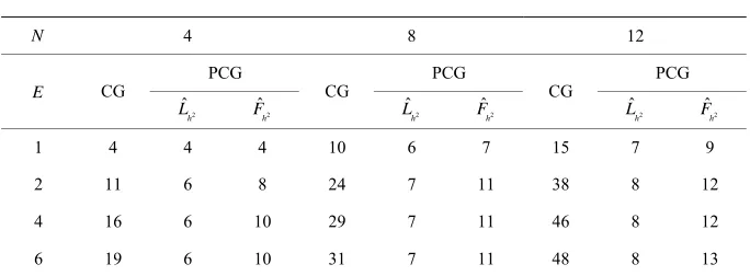
As in the 1D case, we compare the number of PCG it-erations for the preconditioners Lˆh2 and Fˆh2 which
provided [12]. In Table 3, we can see the
sug-gested finite difference preconditioner is more is
in that
2
ˆ
h
L
10−5 100 105 1010
0 20 40 60 80 100 120 140 160 180 200
q
1/p1
Condition number
↓ β = max(1, q
1/4p1)
← β = q
1/4p1
Figure 6. Condition numbers of L Aˆh2ˆh N2 2
1
[image:9.595.312.531.543.708.2]Table 3. Iteration numbers
4 8 12
in 2D.
N
PCG PCG PCG CG
2
ˆ h
L Fˆh2
CG
2
ˆ h
L Fˆh2
CG
2
ˆ h
L Fˆh2
E
1 4 4 4 10 6 7 15 7 9 2 11 6 8 24 7 11 38 8 12 4 16 6 10 29 7 11 46 8 12 6 19 6 10 31 7 11 48 8 13
efficient as compared to the finite element precondi-tioner
Spectral Collocation Approximations to Elliptic Prob-lems,” SIAM Journal on Numerical Analysis, Vol. 32, No.
. 333-385. doi:10.1137/0732015
1
P
2
ˆ
h
F .
6. Conclusion
We have proposed finite differences prec rs and for spectral element discretizations, and c
on LGL nodes for uniformly e ptic pr
n-d ension, , resp ively. he tw o
tioners optim he c ponding spectral ele ments problems was emonstrated th ugh the theor cal proofs and the c putational res s. Th rden the efficiency is now on t ultigrid algorithm for solving finite-differe es pr ms and not G
igh-order elements.
REFERENCES
nd E. H. Mund, “Finite Element Precondi-ob
put
onditione Lˆh
in n
2
ˆ
h
L structed
im
on-lli oblem
n1,ality for t
2 ect
orres
T o prec di
d ro
eti-om ult e bu of
he m oble
nc on M for
h
[1] M. O. Deville a
tioning for Pseudospectral Solutions of Elliptic Pr -lems,” SIAM Journal on Scientific and Statistical
Com-ing, Vol. 11, No. 2, 1990, pp. 311-342.
doi:10.1137/0911019
[2] S. D. Kim and S. Parter, “Preconditioning Legendre spec-tral Collocation Method for Elliptic Partial Differential Equations,” SIAM Journal on Numerical Analysis, Vol.
33, No. 6, 1996, pp. 2375-2400.
doi:10.1137/S0036142994275998
[3] S. D. Kim and S. Parter, “Preconditioning Chebyshev Spectral Collocation by Finite Difference Operators,”
SIAM Journal on Numerical Analysis, Vol. 34, No. 3,
1997, pp. 939-958. doi:10.1137/S0036142995285034
[4] S. Parter, “Preconditioning Legendre Spectral Collocation Methods for Elliptic Problems I: Finite Difference Op-erators,” SIAM Journal on Numerical Analysis, Vol. 39, No. 1, 2001, pp. 330-347.
doi:10.1137/S0036142999365060
[5] S. Parter, “Preconditioning Legendre Spectral Collocation Methods for Elliptic Problems II: Finite Element Opera-tors,” SIAM Journal on Numerical Analysis, Vol. 39, No.
1, 2001, pp. 348-362. doi:10.1137/S0036142999365072
[6] S. Parter and E. Rothman, “Preconditioning Legendre
2, 1995, pp
[7] A. Quarteroni and E. Zampieri, “Finite Element Precon-ditioning for Legendre Spectral Collocation Approxima-to Elliptic Equations Systems,” SIAM Journal umerica lysis, Vol. 29, No. 4, 1992, pp. 917-936. doi:10.1137/072
tions
on N
and
l Ana 9056
[ S. A rszag pectra ethod or Problems in Com-plex omet Journal of Co utational Physics, Vol.
37, 1, 19 .
doi:10.1016/0021-9991(80)90005-4
8] . O Ge
, “S ries,”
l M s f
mp
No. 80, pp. 70-92
[ J. H , T. Manteuffel, S. McCormick and L. Olson, “Algebraic Multigrid (AMG) for High-Order Finite Ele-ments,” Journal of Computational Physics, Vol. 204, No. 2,
9] eys
2005, pp. 520-532. doi:10.1016/j.jcp.2004.10.021
[10] P. Fischer, “An Overlapping Schwarz Method for Spec-tral Element Solution of the Incompressible Navier-Stokes equations,” Journal of Computational Physics, Vol. 133,
No. 1, 1997, pp. 84-101. doi:10.1006/jcph.1997.5651
[11] J. W. Lottes and P. F. Fischer, “Hybrid Multigrid/Schwarz Algorithms for the Spectral Element Method,” Journal of Scientific Computing, Vol. 24, No. 1, 2005, pp. 45-78. doi:10.1007/s10915-004-4787-3
[12] S. D. Kim, “Piecewise Bilinear Preconditioning on High- Order Finite Element Methods,” Electronic Transactions on Numerical Analysis, Vol. 26, 2007, pp. 228-242.
[13] S. Kim and S. D. Kim, “Preconditioning on High-Order Element Methods Using Chebyshev-Gauss-Lobatto Nodes,”
Applied Numerical Mathematics, Vol. 59, No. 2, 2009, pp.
316-333. doi:10.1016/j.apnum.2008.02.007
[14] C. Canuto, M. Y. Hussaini, A. Quarteroni and T. A. Zang,
Dynamics,” Springer, New York,
ible Fluid Flow,” In: Cam-omputational Mathe-
“Spectral Methods: Fundamentals in Single Domains,” Springer, New York, 2006.
[15] C. Canuto, M. Y. Hussaini, A. Quarteroni and T. A. Zang, “Spectral Methods: Evolution to Complex Geometries and Applications to Fluid
2007.
[16] M. O. Deville, P. F. Fischer and E. H. Mund, “High-Or- der Methods for Incompress
bridge Monographs on Applied and C