Munich Personal RePEc Archive
Model uncertainty and expected return
proxies
Jäckel, Christoph
Technical University Munich
5 December 2013
Online at
https://mpra.ub.uni-muenchen.de/51978/
Model uncertainty and expected return proxies
Christoph J¨
ackel
∗First draft: November 18, 2013
This draft: December 5, 2013
Abstract
Over the last two decades, alternative expected return proxies have been proposed with substantially lower variation than realized returns. This helped to reduce parameter uncertainty and to identify many seem-ingly robust relations between expected returns and variables of interest, which would have gone unnoticed with the use of realized returns. In this study, I argue that these findings could be spurious due to the ig-norance of model uncertainty: because a researcher does not know which of the many proposed proxies is measured with the least error, any infer-ence conditional on only one proxy can lead to overconfident decisions. As a solution, I introduce a Bayesian model averaging (BMA) framework to directly incorporate model uncertainty into the statistical analysis. I employ this approach to three examples from the implied cost of capital (ICC) literature and show that the incorporation of model uncertainty can severely widen the coverage regions, thereby leveling the playing field between realized returns and alternative expected return proxies.
Keywords: Time-varying expected returns, implied cost of capital, asset pricing, model averaging, model selection
JEL Classifications: G12, C11
1
Introduction
Realized returns are an unbiased, but noisy, estimator of expected returns. The noise, driven by changes in expectations about future cash flows and discount rates, is typically assumed to be an order of magnitude larger than the variation in expected returns. These information surprises make it notoriously hard to
∗
uncover a relation between a variable of interest and latent expected returns, if realized returns are used as proxy.
In his presidential address, Elton (1999) highlighted these points and chal-lenged the profession to propose alternative ways to estimate expected returns. This request has been followed by a large number of studies that propose al-ternative proxies. They are forward looking and therefore, at least in theory, unaffected by any news. They rely on earnings forecasts (see, e.g., Claus and Thomas 2001), CDS spreads (see Friewald et al. 2013), and corporate bond yields (see Campello et al. 2008). Due to their substantially lower standard de-viation in comparison to realized returns, they allow researchers much sharper statistical inferences and provide them with very robust results. In other words, parameter uncertainty is greatly reduced, which has helped to identify relations between expected returns and factors that are overshadowed by noise when realized returns are used.1
In this paper, I argue that the seemingly robust results of these alternative expected return estimates could be driven, at least partly, by the ignorance of model uncertainty. As a solution, I introduce a Bayesian model averaging (BMA) approach that directly incorporates model uncertainty into the statisti-cal inference. This levels the playing field between realized returns, with large parameter uncertainty and no model uncertainty, and alternative proxies, with typically modest parameter uncertainty, but potentially large model uncertainty. I apply BMA to three research questions from the implied cost of capital (ICC) literature and show that the incorporation of model uncertainty can lead to sampling uncertainties in estimated parameters that are no better than those based on realized returns.
There are two channels through which model uncertainty of expected return proxies is introduced. First, every proxy is based on an underlying theoretical framework such as the Merton-model that links debt and equity returns or the dividend discount model that links the current stock prices with future expected dividends. Proxies based on any such model inherit the model’s shortcomings. Second, and more importantly, to get empirically traceable versions of the the-oretical models additional simplifying assumptions have to be made. These problems are best seen in the case of the most successful proxy, the implied cost of capital, which has seen widespread use in both asset pricing and cor-porate finance. Theoretically, the ICC is just the IRR of the classical dividend
discount model. However, expected dividends are as unobservable as expected returns. As such, proxies, such as analyst earnings forecasts, have to be used and terminal value assumptions have to be made about future periods for which those proxies are not available anymore. This has led to the availability of a few dozens alternative ICC implementations, with minor and major modifications. All alternatives want to measure expected returns, yet all alternatives differ, which directly implies that, at the most, one measures expected returns cor-rectly. Therefore, model uncertainty is caused by measurement error. However, there is ample evidence – both theoretical and empirical – that this measure-ment error is persistent and systematic.2 Consequently, this measurement error can systematically bias the results in those cases where it is correlated with the variable of interest. And even if one is willing to assume that measurement error is white noise, there is an increasing chance of finding significant results due to an increasing number of alternative proxies, all with a different measurement error process. This increases the danger of data snooping.
The current approach to deal with this problem is to run robustness tests in an ad-hoc manner. To the best of my knowledge, there is no study that takes the evidence from different proxy classes, i.e. proxies derived from different un-derlying theoretical models, into account. Additionally, most studies that only focus on one proxy class, in almost all cases the ICC, only vary minor specifi-cations of a specific ICC method. Of course, this approach can be justified by the large number of possible specifications that make it hard for the researcher to check for and for the reader to comprehend. Yet, it is well known from the model selection literature that results conditional on only a few models lead to the understatement of predictive and inferential uncertainty about a parameter of interest, “leading to inaccurate scientific summaries and overconfident deci-sions that do not incorporate sufficient hedging against uncertainty” (Draper 1995, p. 45).
However, a solution to this problem is available: Bayesian model averaging, in which an econometrician averages across the evidence conditional on each model. Hereby, the weight of each model is determined by the prior beliefs of the econometrician about the model probability and the parameters, on the one hand, and the evidence in the data, on the other hand. Herein lies the key differ-ence of my implementation of BMA to other studies. In those studies, a model
gets the higher posterior model weight, the better it is able to explain the data at hand, which is a faulty approach in the case of measurement error. Suppose we are interested in the relation between expected returns and any variable of interestx, but only have a set of different proxies for expected returns available. Suppose further that there is no relation between expected returns andx, but between the measurement error of one of the proxies and x. Obviously, this proxy will have the strongest relation with x asymptotically and hence, given the data, it would get the highest weight.
We, therefore, need an external validation of a proxy’s quality. Previous research, such as Easton and Monahan (2005) and Lee, So, et al. (2011), argue that, since realized returns over period t+ 1 are an unbiased estimator of re-turns for that period, expected at time t, any alternative proxy eventually has to explain subsequent realized returns. However, they only use such predictive regressions to identify the best proxy. In contrast, I apply a BMA setup to obtain posterior model weights from predictive regressions. I thereby closely follow Avramov (2002), Cremers (2002), and Binsbergen et al. (2013), who also combine BMA and predictive regressions, but with different goals. Avramov (2002) and Cremers (2002) want to improve the predictive accuracy by combin-ing signals from many predictors. Binsbergen et al. (2013) evaluate the quality of their equity yields in comparison to other predictors. So their approach is similar to mine in that they differentiate between different predictors (in their case) or proxies (in my case). However, they do not use these model weights in a follow-up step. In contrast, the computation of model weights is only an intermediate step in my approach. In a final step, I use the model weights to average across the parameters of interest over all proxies under consideration. If these parameters differ between proxies, this results in larger coverage regions that take model uncertainty into consideration.
any study within the ICC literature that has provided conclusive arguments to favor one specification over another. The same is true for comparisons across proxy classes.
The approach also highlights another problem of alternative expected return proxies. If the true underlying expected return process is not within the set of proxies under examination, results will be biased, even asymptotically. Hence, a model averaging approach can only reduce model uncertainty issues, not solve them.
In summary, the contribution of this paper is twofold: First, it provides a general framework to incorporate model uncertainty into the inference based on expected return proxies. This framework is also very instructive in pointing out the underlying weaknesses of alternative expected return measures other than realized returns: in particular, the inability for a researcher to establish their unbiasedness and the dependency on realized returns to evaluate them. Second, I apply the model averaging framework to three examples based on the time-series of the ICC and show that ignorance of model uncertainty can lead to overconfident decisions. In particular, I find that the recent results of Chen et al. (2013), who use the ICC to answer the question of whether stock price movements are driven by cash flow or discount rate news, are not robust when evidence is based on alternative, reasonable specifications of the ICC.
The rest of the paper is organized as follows. Section 2 shows the problems that are caused by the uncertainty inherent in the proxy selection process and introduces BMA as a possible solution to this problem. Section 3 describes the data set that is used in Section 4 to apply BMA to three examples from the ICC literature. Section 5 concludes.
2
Theoretical considerations
2.1
Theoretical framework
Suppose we are interested if the time-series of variablextis related to expected
returnsEt[rt+1]≡µt. Concretely, suppose the following linear relation:3
µt=γxt+ǫt, t= 1, . . . , T. (1)
Using a univariate, classical regression setting with normally distributed mean zero errors ǫt, we can regress µt on xt and test if the estimator bγ is
signifi-cantly different from zero. However, since µt is unobservable, the researcher
has to identify observable proxies, one of which is realized returns rt+1.
Re-alized returns over a period t+ 1 are the sum of expected returns at time t and unexpected returnsut+1 that have a mean of zero conditional on all of the information available at timet:4
rt+1=µt+ut+1, t= 1, . . . , T. (2)
Given equation (2), it is easily shown that the unconditional mean of rt+1 is equal to the unconditional mean ofµt. In other words, realized returns are an
unbiased estimator of expected returns. Despite this advantageous characteris-tic, realized returns have come under criticism due to the fact that the variation in ut+1 is an order of magnitude larger than the variation in µt. This makes
statistical inference notoriously hard, as highlighted by Elton (1999). Plugging equation (2) into (1), the sampling variance of the estimator based on realized returns,bγrr, is given by:
V ar(bγrr) =
V ar(ǫt) +V ar(ut+1) PT
t=1(xt−E[x])
2 . (3)
In small samples, the large variance ofut+1 results in a large sampling variance forbγrr that can hinder the detection of an existing relation betweenµtandxt.
This insight has led to a “proxy variable search” with the hope of identifying alternative proxies for expected returns that are not plagued with the large noise inherent in realized returns.
However, these proxies are subject to measurement error. In line with previ-ous research (see, for example, Easton and Monahan (2005) and Lee, So, et al. (2011)), I assume that a proxyµbt,k, measured at time t, is trackingµtwith an
additional, additive proxy-specific error term wt,k:
b
µt,k =µt+wt,k, t= 1, . . . , T. (4)
3. For simplicity, I assume the intercept to be zero.
If we run regression (1) with a proxy as defined in equation (4), it can be shown that the resulting regression coefficientbγk is equal to the sample estimate that
we would obtain ifµtwere observable, bγ, and an additional bias term:
b
γk =bγ+Cov(wt,k, xt)
V ar(xt)
=bγ+Biask. (5)
Obviously, the hope of a researcher who applies proxy k is that the mean and variance of wt,t are close to zero. In this case, the researcher is able to detect
a relation between xt and µt much more precisely, compared to the analysis
that employs realized returns. The danger, however, is quite obvious as well: if wt,k is systematically correlated withxt, or if by chance the two comove in
sample, then one might incorrectly deduce a relation between µt and xt from
the data, although this relation is solely due to the specific measurement error of the proxy under consideration.
Studies such as Easton and Monahan (2005) and Lee, So, et al. (2011) offer a first step to address this problem. They realize that we need an external
validation of the quality of alternative proxies. If we can establish that some of the proxies are unsuitable to track expected returns, we can dismiss them from the beginning. Fortunately, such an external validation is available. Since realized returns over a period are an unbiased estimator of the expected return at the beginning of this period, every reasonable alternative proxy has to be able to predict them eventually. Consequently, predictive regressions such as in Li et al. (2013) provide evidence of the quality of expected return proxies. Therefore, these studies recommend selecting proxies that perform best in such predictive regressions.
However, it is well known from the return predictability literature that pre-dicting subsequent realized returns is notoriously hard. Until now, there is still a heated debate ifany predictor, not just expected return proxies, can actually predict realized returns.5 In summary, we have a large number of proxies to choose from and we are unable to precisely determine which of these proxies is best. Therefore, we face large model uncertainty and the main contribution of this paper is to introduce model averaging techniques, that have been used with great success in different settings, to the expected return proxy literature. The next section shortly introduces model averaging and applies it to the problem at hand.
2.2
Model averaging approach
Within a Bayesian framework, Leamer (1978) shows that the posterior distribu-tion of a quantity of interest ∆ can be computed, given dataD, as the average of the posterior distributions under each model, weighted by their posterior model probability.6
If we interpret each proxy as a separate model, we therefore get:
p(∆|D) =
k X
i=1
p(Mi|D)p(∆|D, Mi), (6)
where M1, . . . , Mk are the models considered. Equation (6) implies that the
marginal distribution of the parameter of interest is a mixture distribution. The mixture probabilities are the posterior model weights, p(Mi|D), and the
individual distributions are the distributions of the parameter of interest, con-ditional on a specific model.
In this simple framework, the only difference between two modelsMiandMj
is that the proxybµiis replaced withµbj.7 Additionally,Dis split into two parts
here: the partDRQis the part of the data needed to answer the research question
at hand. In the simple setup introduced in the previous section,DRQ consists of
the matrix of expected return proxies andxt. DP is the part of the data needed
to compute the posterior probability of each proxy measuring true expected returns, given that one of the proxies is indeed correct. As argued before, this data consists of the set of proxies under consideration and subsequent realized returns. The separation of the data set is a direct consequence of the previous discussion: if we evaluate the quality of a proxy in terms of how well it explains the research question at hand, we run the risk of finding spurious relations driven by measurement error, and not by true expected returns. This is the main differentiation between my approach and other studies that apply BMA: Since measurement error is not such an obvious problem in other studies, a model is considered to be superior if it is able to explain the research question at hand better.8 In contrast, I use subsequent realized returns to infer the posterior
6. The most popular derivative of model averaging is the one based on Bayes’ theorem, which is also the foundation in Leamer’s work. This approach subsumes under the name of Bayesian model averaging. However, there are also frequentist alternatives based on information-theoretical criteria such as AIC or BIC (see Claeskens and Hjort 2008). As I show later on, due to the simplicity of my setup both approaches yield identical results. Therefore, the debate about differences between the two approaches is not an issue for the purpose of this paper. Still, in line with most studies that focus on model averaging techniques, I use a Bayesian setting to motivate my approach.
7. This is important for the reader to keep in mind because I use the words proxies and models somewhat interchangeably. The latter is often used to conform with the language of the model selection and averaging literature.
model weightsp(Mi|DP), which is a measure of the quality of the proxy.9 This
computation is independent of the specific research question. Results for each proxy are then obtained for the research question at hand and averaged across the proxies based on the model weights.
To emphasize the separation between model computation and subsequent statistical inference, equation (6) can be rewritten as:
p(∆|DRQ, DP) = k X
i=1
p(Mi|DP)p(∆|DRQ, Mi). (7)
In principle, the posterior distribution of the parameter of interest,p(∆|DRQ, Mi),
can be derived from a Bayesian perspective. That is, one would specify the prior for this parameter, p(∆|Mi), and the likelihood conditional on the parameter,
p(DRQ|∆, Mi). The posterior is proportional to the product of likelihood and
prior. While this seems to be a daunting task at first glance, it is greatly sim-plified by the fact that each model has the same interpretation in the case of expected return proxies. Since each proxy wants to measure the same thing without error, all parameters should have the same interpretation. In this pa-per, I choose a simpler approach that is more in line with current practice that mostly applies frequentist approaches: For the posterior distribution of the pa-rameter of interest I use the sampling distribution from the frequentist approach. For example, if we run a time-series regression as specified in (1) and are inter-ested in the slope coefficient,p(∆|DRQ, Mi) is just the sampling distribution of
the slope coefficient from a regression of a specific proxy onxt. These
distribu-tions are easily adjusted to incorporate heteroskedastic or autocorrelated error structures, as will be shown in the empirical examples later on.
Coming back to the research question from the previous section, the first two moments ofbγ can then be calculated as:10
E[bγBM A|DRQ, DP] = k X
i=1
p(Mi|DP)bγi, (8)
how to take issues of model uncertainty into consideration. In this application problems of measurement error are ignored. As a consequence, the better a model explains the dependent variable, the higher its posterior model probability will be.
and
V ar(bγBM A|DRQ, DP) = k X
i=1
p(Mi|DP)V ar(bγi|DRQ, Mi)+
+
k X
i=1
p(Mi|DP)(bγi−E[bγBM A|DRQ, DP])2. (9)
While the mean estimate across all models is simply a weighted average across the estimate of each model, the variance of the combined estimate bγBM A
ex-ceeds a weighted average of the variances of the estimates within each model
by an amount that depends on the variability of the estimates across models. Consider a case in whichV ar(bγi|DRQ, Mi) is quite small for all models, i.e.
con-ditional on a certain model the regression coefficient is measured accurately, but across models, the coefficients vary widely. In such a case, one would severely underestimate the variability of the parameter of interest if one only focuses on one model.
In the case of the proxy literature, it is an apparent advantage (see, for instance, Lee, Ng, et al. (2009)) that the statistical inference is much more robust due to much lower standard errors. This statement, however, is often based on evidence for one proxy. Equation (9) shows that the variance could indeed be much larger if the coefficients between different proxies differ substantially.
By plugging equation (5) into equation (8) and (9) and rearranging, we can expressE[γbBM A|DRQ, DP] andV ar(bγBM A|DRQ, DP), respectively, as follows:
E[γbBM A|DRQ, DP] =bγ+BiasBM A, (10)
and
V ar(bγBM A|DRQ, DP) = k X
i=1
p(Mi|DP)V ar(γb+Biasi)
+
k X
i=1
p(Mi|DP)(Biasi−BiasBM A)2, (11)
where BiasBM A =Pki=1p(Mi|DP)Biasi. Equation (10) and (11) are instruc-tive representations of the discussion above. First, if one of the proxies is mea-sured without error, we want the posterior model probability of this proxy to approach unity. In this case,E[bγBM A|DRQ, DP] andV ar(bγBM A|DRQ, DP) will
model uncertainty that is automatically incorporated into the BMA analysis. In contrast, if an econometrician only examines a subset of the proxies, one might end up with biased estimates. Third, if all proxies under consideration are systematically biased, BMA will fail.11
Finally, all approaches that base their results on only one proxy, whether this proxy is chosen ad-hoc or by its ability to predict subsequent realized returns, ignore the variability of the pa-rameters from different models. This leads to overoptimistic decisions and can result in the false identification of seemingly robust relations.12
2.3
Computation of posterior model weights
I follow Avramov (2002), Cremers (2002), and Binsbergen et al. (2013), which are all studies that run predictive regressions in a BMA framework to com-pute posterior model weights. Consider a set of k linear univariate models M1, . . . , Mk. Let the ith model be given by:
rt+1=β0+β1µbt,i+εt+1, t= 1, . . . , T, (12)
whereεt+1is assumed to be identically, independently, and normally distributed with mean zero and unknown variance σ2. In general, the posterior model probability for modeliis computed, given dataDP, via Bayes’ theorem as:
p(Mi|DP) =
p(DP|Mi)p(Mi) P
kp(DP|Mk)p(Mk)
, (13)
where
p(DP|Mi) = Z Z
p(DP|βi, σ2, Mi)p(βi|σ2, Mi)p(σ2)dβidσ2. (14)
Therefore, we have to specify two priors. First, a prior about the probability of each model, p(Mi). Second, priors about the parametersβ = (β0, β1) and σ2
. Both cases can be tricky if the number of explanatory variables differs
11. Therefore, it is a commonly made assumption in the BMA literature that the true model is part of the set of models considered.
between models and if the parameters’ interpretation changes from model to model.13 In my case, however, this is not an issue because each model has only one explanatory variable and the interpretation in each model is the same. The default assumption aboutp(Mi) is to give each model the same weight a priori,
i.e.:
p(Mi) =
1
k. (15)
I use the same priors as Wright (2008) and Binsbergen et al. (2013). Concretely, I make the assumption thatβ takes the natural conjugate g-prior specification proposed by Zellner (1986). The prior on β conditional on the variance of the error termσ2 is therefore given asN(0, φσ2(X′
iXi)−1), whereφ is a shrinkage
parameter that controls the informativeness of the prior and Xi is the T ×
2 matrix of a T vector of ones and the T vector µbi. Since σ2 is identical
across models, we can use an improper prior of an inverse gamma (0,0) that is proportional to 1/σ. Then, the posterior model weights can be computed from:14
p(Mi|DP)∝
r′
r−
φ 1 +φ
r′
Xi(Xi′Xi)−1Xi′r −T /2
, (16)
where r ≡ (r2, . . . , rT+1) denotes the vector of subsequent realized returns.
Finally, we just have to normalize equation (16) so that all model weights sum to one.
The parameterφgoverns the informativeness of the researcher’s prior infor-mation. The lowerφ, the more weight is put on prior information. In the limit, if φ= 0, p(Mi|Dp) is equal for all models, i.e. the posterior probabilities are
identical to the prior probabilitiesp(Mi).
To provide a link with frequentist approaches and to get rid of the subjective aspects of the prior assumptions, we can increaseφto reduce the impact of the priors. In the limiting case, i.e. φ→ ∞, the posterior model weights in equation (16) become proportional to (SSE)−T /2. This result is also derived by Leamer (1978, p. 112) who is in search of a reasonable diffuse prior. Furthermore, it is easy to show that in this case the weights computed from equation (16) are identical to the weights that would be obtained from information-theoretical approaches that use AIC or BIC based on the following formula:15
pAIC(i) =
exp(0.5∆AIC,i) P
kexp(0.5∆AIC,k)
, (17)
where ∆AIC,k =AICk−maxAIC. This subtraction is made merely for
com-13. For a discussion of these issues, see, for instance, Ley and Steel (2009).
14. I can ignore all terms here that are constant across models because they cancel out in equation (13).
putational reasons. In equation (17), we can replace AIC with BIC; since the model sizes are identical across models, the penalty term that normally differs between AIC and BIC does not matter.
To summarize, both a noninformative Bayesian approach as well as a fre-quentist approach yield identical results due to the simplicity of the setup (uni-variate linear regression for each model). Consequently, debates about which approach is superior are not relevant here and model weights, given the data, are easily computed. The better a proxy is able to explain subsequent realized returns, i.e. the lower the sum of squared errors is in the predictive regression, the more credible this proxy is in comparison to its competitors and the more weight a researcher should assign to it in the analysis of interest.
Due to the high level of noise inherent in realized returns, alternative proxies have been proposed. That is, the main motivation for these proxies is the re-placement of realized returns. However, the previous analysis to infer the quality of these proxies has to rely again on the very same realized returns it wants to replace. In my opinion, this is a severe shortcoming ofanyalternative expected return proxy, a point that has mostly gone unnoticed in the literature.16
A main contribution of this study is that the introduction of model averaging techniques allows me to shed light on this issue. For the sake of simplicity, let’s focus only on two alternative proxies with equal prior probability. In this case, the Bayes Factor and the likelihood ratio (again, they are identical due to the simplicity of the setup) can be interpreted as a summary of the evidence provided by the data in favor of one proxy, in comparison to another proxy.17
In our case, the Bayes Factor is given by:
BF12=
SSE2 SSE1
T /2 =
V ar(wt,2) +V ar(ut+1)
V ar(wt,1) +V ar(ut+1) T /2
. (18)
As argued above, the main motivation of any alternative proxy is the large variation in realized returns induced byut+1. Thus, equation (18) will be
dom-inated by the term V ar(ut+1), which means that in small samples it will be
notoriously hard to separate proxies with low measurement error from proxies with large measurement error. This means that the weights will not converge quickly to the best proxies in small samples. Only if sample size increases, even
16. I am only aware of Guay et al. (2011, p. 129), who give a qualitative assessment of this issue: “Like Easton and Monahan (2005) and a large literature in finance, we use realized returns as a metric to assess the cost of capital estimates and the effectiveness of our proposed remedies. Although our returns-based tests are consistent with a large asset-pricing literature, we acknowledge that realized returns are a noisy proxy for expected returns, and that this is, in fact, an important motivation behind implied cost of capital measures. However, despite the limitations, we are unaware of a superior benchmark to validate cost of capital measures that does not rely on realized returns.”
SSE ratios close to one will eventually become large and reveal the superiority of one proxy over the other. Furthermore, it is often argued that ut+1 can be correlated with other variables in sample and therefore, inferences based on it can be misleading.18
As a consequence, in small samples it might happen that inferior proxies get more weight.
3
Proxy selection and data
In general, the BMA approach can be applied to any empirical proxy of expected returns. However, the only proxy that has found widespread use in empirical applications so far is the ICC. Probably as a result of this success, it is also the only proxy with a multitude of alternative versions, which emphasizes the im-portance of incorporating model uncertainty into the empirical analysis. Hence, I focus on the ICC in the empirical part of my study.
The ICC is defined as the constant discount rate rICC that equates the
current stock price of firmi,Pi,t, with the sum all future dividends, discounted
to today:
Pi,t=
∞
X
j=1
Et[Di,t+j]
(1 +ri,ICC)j
, (19)
whereEt[Di,t+j] denotes the dividend in period t+j that the investor
ex-pects at t. To get empirically traceable versions of equation (19), certain sim-plifying assumptions have to be made by the researcher, thereby introducing model uncertainty. Since market expectations about future dividends are just as unobservable as expected returns, proxies have to be used. The most com-mon ones are analyst forecasts forearnings that I use here as well.19
Since the dividend discount model of equation (19) can be transformed into a model that takes earnings as an input in several ways, this is a first differentiator between ICC methods: while derivatives of the residual income model rely on the
clean-18. Fama and French (2002), for instance, argue that the high realized returns in the U.S. stock market in the second part of the twentieth century were a result of a series of positive cash flow news that generated positive shocksut+1and not a result of highµtfor this period. Additionally, Campello et al. (2008) also run the predictive regressions of their expected re-turn proxy and do not find a large explanatory power of their proxy. Instead of attributing this result as a negative sign for the quality of their proxy, they blame the shock structure in the sample for this result and conclude that it is therefore worthwhile to explore alternative proxies. Yet another indication of the sensitivity of the specific sample is the evidence pre-sented in Koijen and Van Nieuwerburgh (2011) that the regression coefficients in predictive regressions are instable over time.
surplus relation to link dividends to earnings and book values, the abnormal growth in earnings model does not have to rely on book values.20 Another distinguishing feature between ICC methods is their terminal value assumption that has to be made since earnings forecasts are only available for the next few years.
[Table 1 about here.]
In this paper, I focus on two derivatives of the abnormal growth in earnings model (OJ, MPEG), two derivatives of the residual income model (GLS, CT), and two direct implementations of equation (19) (PSS, CDZ) that have found widespread use in the literature. Table 1 presents the different methods and the specific assumptions made by them.
All methods rely on analyst forecasts, which are obtained monthly from IBES. IBES provides analyst forecasts for up to five years ahead, but mostly only the first two to three years are covered. Missing earnings forecast from periodt+ 3 on are filled up by multiplying the forecast of the previous year and the long-term earnings growth rate provided by analysts: epsi,t+j=epsi,t+j−1× (1 +Ltgt). IBES also provides the stock price, the shares outstanding, and
a long-term growth rate Ltg. I match this data with data from Compustat that is publicly released. From Compustat, I obtain shareholder’s equity (item SEQ) and common shares outstanding (item CSHO) to infer the book value per share.21 Also, the payout ratios for the next three years are assumed to be constant and equal to the historical one, i.e. I divide common dividends (item DVC) by income before extraordinary item (IBCOM). For firms with a negative income, 6% of total assets is used as the denominator instead. With this data and further assumptions described in Table 1, I can solve numerically for the value of the ICC that sets the difference of the current price and discounted dividends to zero. I abort the root search as soon as the change in the ICC is less than 0.001% for one step. The ICC is computed at the IBES release date which is on the Thursday before the third Friday in each month. I match the ICC of this date with subsequent realized returns of the next calendar month.22 The realized returns are the continuously compounded with-dividend monthly returns on the value-weighted portfolio of all NYSE, Amex, and NASDAQ stocks from the Center for Research in Security Prices (CRSP).23
20. Easton (2007) gives an introduction into the various ICC methods and their assumptions. 21. The reason I obtain shares outstanding both from Compustat and IBES is that the former is used to match it consistently to the historic shareholder’s equity, while the latter is used to compute the monthly updated market capitalization. Calculating the market capitalization of a firm as the product of the IBES price and shares outstanding is common practice in the literature.
22. In untabulated results, I also compute monthly returns from the IBES release date to the day before the next IBES release date, which only has a marginal effect on the results.
I filter all observations that have at least one missing value of an ICC method, that have a negative book value and that have an IBES price below one dollar. With the remaining observations, I compute a monthly, value-weighted time-series for each ICC method from 1985 to 2011.
Note that the studies referred to in column 2 of Table 1 are the reference points for my procedures. This does not mean that I replicate their approaches exactly. For better comprehensibility, I reduce the assumptions made by the cited studies to a common denominator. For instance, empirical studies differ on how they fill up missing analyst forecasts. Some studies require at least three forecasts to be available, some studies use the long-term earnings growth rate to compute missing forecasts, and some studies compute this growth rate, if missing, from available earnings forecasts. Also, applied filters differ from study to study. Here, I apply the same rules of inferring missing data and filtering, as described above, consistently to all methods.
While the arbitrary decisions about issues discussed in the previous para-graph should have a negligible effect on the results, the column 4 in Table 1 shows assumptions that should have a far more pronounced impact. For in-stance, the MPEG and OJ method only rely on analyst forecasts for the next two periods, while the CT method takes the forecasts of all five years ahead into account. GLS, PSS, and CDZ use the first three forecasts. These methods also differ substantially in their terminal value assumptions: GLS linearly interpo-lates the three-year ahead ROE to the historical median industry ROE over the next nine years. In contrast, PSS and CDZ use an exponential rate of decline to mean-revert the year t+ 3 earnings growth rate gt+3 to a long-run growth rate in yeart+ 16,gLT. While the PSS method assumes that this growth rate
is equal to the steady-state growth rateg, which is set to the historical average of the long-run nominal GDP growth rate, the CDZ method breaks this link between the long-run growth rategLT and the steady-state growth rateg. The
former is set to the mean long-term analyst industry growth forecast, the latter is identical togin the PSS case.
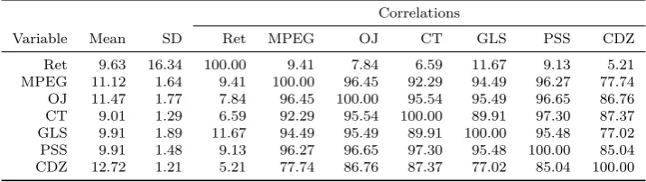
[Table 2 about here.]
Table 2 presents summary statistics for the ICC methods and realized re-turns. In line with previous research, all ICC methods have standard deviations that are an order of magnitude smaller than the standard deviation found in re-alized returns, which is considered to be one of the latter’s main disadvantages. For example, Lee, Ng, et al. (2009) label realized returns an extremely noisy
ICCs, i.e. implied risk premiums, to predictexcessrealized returns to be consistent with prior
proxy for expected returns and Table 2 confirms this view. The large noise in realized returns is also a driver of the low correlation between realized returns on the one hand and all ICC methods on the other hand. Nevertheless, all corre-lations are at least positive, a result that does not hold in the cross-section (see for example Easton and Monahan (2005)). Since all variables measure expected returns in theory, a positive correlation between those variables is confirmative, albeit weak, evidence that this is indeed the case. The correlation between the ICC methods is almost perfect, which contrasts evidence in the cross-section. This supports the view of Li et al. (2013) who claim that the aggregate ICC is less likely to be noisy because estimation errors present in firm-level ICCs are reduced through averaging. This result also implies that model uncertainty is far less an issue in the time-series than in the cross-section. Nevertheless, even in the time-series a researcher who wants to use the ICC in the empirical analysis will face quite some model uncertainty. First, while most of the cor-relation coefficients are over 90%, they are as low as 77%. Second, the mean across different ICC methods varies from 9.01% for method CT to 12.7% for method CDZ. Noteworthy differences are also present in the standard deviations of the various ICC methods. It becomes clear from Table 2 that a researcher would severely underestimate the true uncertainty in the statistical inference if he would base the results solely on one method. In this case he would focus on parameter uncertainty only, thereby completely ignoring model uncertainty.
4
Empirical results
4.1
Weights
[Table 3 about here.]
Table 3 shows the posterior model weights that are obtained from applying equation (16) with different shrinkage parameters φ. As has been argued in Section 2, a shrinkage parameter close to zero puts almost all weight on prior information and leaves little room for the data to change the researcher’s view on his priors. Since the priors are equally weighted across models, so are the posteriors in the case ofφ= 0.01.
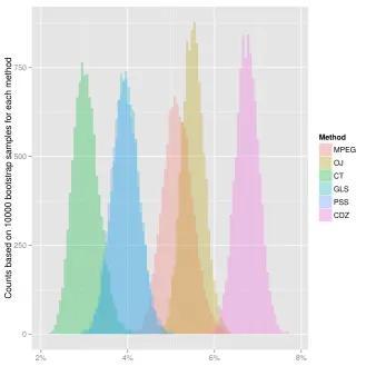
The moreφis increased, the more weight is put on the evidence in the data. And for this particular data set, the GLS method is performing best in predicting subsequent realized returns. In the limiting case in which the researcher discards all prior information (φ=∞), the posterior model weight of the GLS method is 39%. The ordering of the methods can also be inferred from the correlations between the ICC methods on the one hand and subsequent realized returns on the other (see Table 2). The higher the correlation, the higher the R2, and the lower the sum of squared errors. And this is just the criterion to transform evidence in the data into model weights. Furthermore, it is interesting to see that the CDZ method gets almost no support from the data.
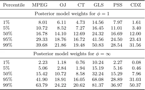
[Table 4 about here.]
How robust are these posterior model weights though? Table 4 gives the answer to this question. It shows the distribution of the posterior model weights for two different shrinkage parameters (φ = 1 and φ = ∞) and for 10,000 bootstrap runs. In each run, a random sample with replacement and the same size as the original data set (i.e. 324 months) is drawn and the posterior model weights are computed for this bootstrap sample.
To determine the quality of any such proxy, one needs the very same realized returns it ought to replace.
The large noise in realized returns and its consequences are well known in the finance literature. Goyal and Welch (2008) argue that apparent statistical significance of many predictors are exclusively due to years up to and especially on the years of the Oil Shock from 1973 to 1975. Fama and French (2002) find that the high realized returns of the second half of the 20th century are mostly driven by positive unexpected shocks, and not by high expected returns. And Campello et al. (2008) run the predictive regressions from above with their expected return proxy based on yield spreads and find no relation. They interpret this result as evidence that the shock structure in realized returns in their sample hindered the convergence to their expected return proxy, assumed to be correct, not as evidence that their proxy might be measured with error. From the perspective of the BMA approach advocated here, they have a very informative prior about the correctness of their proxy and therefore, discard any information in the data that casts doubt on this prior.
However, this leaves only one way to evaluate the performance of any proxy, that is, prior information. Of course, since in most empirical studies only one proxy class is under consideration, the implicit weight on this proxy is set to one. But this severely overstates, at least in my opinion, the confidence a researcher should have in his proxy. In the example of Campello et al. (2008), if their proxy is not able to explain subsequent realized returns, why should I choose their proxy instead of ICCs or proxies based on CDS spreads? In other words, a researcher who proposes a new proxy has to compare this proxy with existing ones. The only meaningful method of comparison that I know of are predictive regressions that are highly sensitive, so that a researcher might ignore these regressions altogether. But in this case, the researcher has to choose between two options. Either he considers evidence of all proxies simultaneously, which will weaken the power of statistical tests and therefore reduce one of the main advantages of alternative expected return proxies. Or he argues based on prior information why he deems his proxy more suitable than others and he has to quantify the superiority of his proxy.
has no reference for which of these variations is most supported by the data. It is also hard for him to combine the evidence from the battery of robustness tests to one coherent picture. And finally, the variations chosen in the robustness section are mostly chosen ad-hoc with no evident motivation. This is nicely illustrated in the ICC literature. Most asset pricing studies focus on the PSS approach and its derivatives, while most corporate finance studies implement abnormal growth in earnings models and residual income models. Newer studies mostly focus on one approach and change some input parameters, ignoring evidence based on other approaches. This procedure could be motivated by the fact that too many robustness checks will unnecessarily lengthen the paper and bore the reader, especially if the results are quite similar. However, as I show in subsequent examples, omitting such tests can result in quite dramatic misinterpretations.
The model averaging approach proposed in this paper is a solution to this problem. If a researcher is willing to make the extra effort to motivate this approach shortly, model averaging can take any number of expected return proxies into account without increasing the complexity of the analysis. Also, it automatically incorporates evidence about the quality of the proxies under consideration, if one is willing to take predictive regressions, despite their sen-sitivity to large shocks, into account. So if one proxy class gets no support in the data, it will not matter in the following empirical analysis. The weight-ing between the prior information and the data can easily be controlled by the researcher. Furthermore, this approach helps to protect a researcher of find-ing spurious relations between the variable of interest and expected returns by making sure that a researcher is not just selecting a proxy with a particular measurement error process that is related to the variable of interest. However, even this approach is not able to solve the problem of whether any proxy is tracking expected returns well. If no proxy does, the analysis will still be bi-ased, even asymptotically. This is a severe shortcoming of any expected return proxy. Finally, the BMA approach subsumes current approaches, which also apply a model averaging approach implicitly by setting the probability of one proxy to one. So it is also possible to replicate current studies exactly with my approach. However, it requires the researcher to explicitly state his prior.
In the following, I present three empirical examples that show the impact of model uncertainty and apply the model averaging approach to deal with it.
4.2
The implied equity risk premium
research. They use the ICC to compute an implied risk premium, defined as the ICC minus the 10-year government bond yield, and find that the U.S. implied risk premium is only around 3% from 1985 to 1998. Due to a lack of alternative proxies back then, they only apply the CT approach.
I replicate their analysis for an updated time period from 1985 to 2011 and also incorporate model uncertainty into the analysis by considering six ICC methods simultaneously. In this example, I set φ= 0, i.e. I consider each ICC method equally likely to track expected returns correctly. Hence, the posterior model weights are equal to the prior model weights; each ICC method gets the same weight. The reason why I do not consider the evidence from predictive regressions as relevant for this research question is because I assume that the level of the ICC, in which we are interested in here, is unrelated to the time-series process of the ICC. Only the latter is evaluated with predictive regressions, but since I assume that there is no relation to the former, these regressions do not help me in differentiating between the different methods. As a simple example, take two proxies, one that tracks expected returns perfectly, but is 10% too high every period, and one that is either 2% too high or 2% too low, with equal probability. While the former proxy is biased in levels, it will perfectly track the time-series of expected returns. The latter, on the other hand, will be unbiased, but not track expected returns reasonable well. In this application, we want to choose the latter, but the predictive regression would choose, at least asymptotically, the former. Hence, I ignore it.
[Figure 1 about here.]
Two additional points are worth repeating here. First, model uncertainty is not completely eliminated. For instance, all proxies are based on analyst forecasts and these forecasts are probably biased upwards. Of course, one could also adjust the model weights based on prior information. For example, the assumption made in the CDZ method that earnings grow with the analysts’ long-term growth rate until year 15 is certainly a very aggressive growth assumption. If one deems this assumption to be unreasonable, the prior model weights of the method can be reduced accordingly. Second, this example still proves the usefulness of alternative proxies. The six ICC methods cover a wide range of earnings growth assumptions and yet, the results imply that the implied risk premium is positive and lies within a realistic range. Such a statement cannot be made for such a short period based on realized returns. Therefore, the increase in the variance, due to model uncertainty, is still considerably lower than the decrease, due to eliminating the large shocks that affect realized returns.
4.3
The intertemporal risk-return tradeoff
Although finance theory predicts a positive risk-return relation, empirical evi-dence based on realized returns does not conclusively find a positive sign. In simulations, Lundblad (2007) shows that even if there is a positive relation be-tween the conditional variance and the conditional expected return, it takes very long samples to identify this relation with noisy realized returns.
Consequently, P´astor, Sinha, et al. (2008) replace realized returns with an ICC measure estimated with the PSS method. They find a positive relation between the conditional mean of market returns, approximated by their ICC, and the variance of market returns for the years 1981 to 2002. Empirically, they run the following regression specifications, which I replicate and extend with the model averaging approach:24
b
µt=a+bV olt+et (20)
∆µbt=a+b∆V olt+et, (21)
whereµbtis a proxy for expected excess returns andV oltis either the annualized
variance or standard deviation of the daily value-weighted market returns from CRSP for this period. Since the IBES release date is typically a few days after the 15th of each month, I compute the conditional volatility based on returns ranging from the first trading day after the 15th of the previous month to
the first trading day after the 15th of the current month.25 The implied risk premiums are the difference between the ICC minus the 10-year government bond yield. ∆bµt and ∆V olt are the first difference of the conditional market
return mean and volatility proxies, respectively. Because the ICC is highly persistent, I follow P´astor, Sinha, et al. (2008) and use 12 Newey-West lags in regression (20). Since the first difference of ICCs does not show a persistent autocorrelation structure, they and I use one lag for specification (21).
[Table 5 about here.]
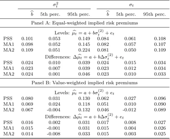
The rows labelled “PSS” in Table 5 repeat the analysis of P´astor, Sinha, et al. (2008) for a different time period (1985 to 2011 instead of 1981 to 2002). Despite the different time periods, the results are very similar. Like them, I find a positive risk-return tradeoff for both the levels and the first difference regressions and for equally and value-weighted implied risk premiums. These results are also robust: the 5th percentile based on Newey-West corrected standard errors is positive in all specifications.
In rows “MA1” and “MA2”, I apply the model averaging approach to check whether these robust results could be overestimated due to the ignorance of model uncertainty. Since the density of the slope coefficientbb, conditional on a specific ICC method, follows a t-distribution, the density across models is a weighted average of these conditional densities. This is simply a mixture t-distribution from which I sample 1,000,000 times. As a robustness check, I also implement a second model averaging approach, MA2, in which I generate 60,000 block-bootstrap samples with a block length of 24 months for equation (20) and 3 months for equation (21). In each sample, an ICC method is chosen randomly based on the posterior model weights. For this example, I decide to use a diffuse prior and setφto∞.
Table 5 shows that the consideration of model uncertainty has a negligible effect on the results. In all specifications, the mean of the sampled coefficients is very similar to the regression coefficient from the PSS case. Also, the 90% coverage region widens only marginally. There are now some cases in which 5% of the drawn coefficients are negative, but by and large almost all draws across the eight specifications are positive. This confirms the findings of P´astor, Sinha, et al. (2008) that there is a positive relation between the conditional market return and the conditional volatility.
[Figure 2 about here.]
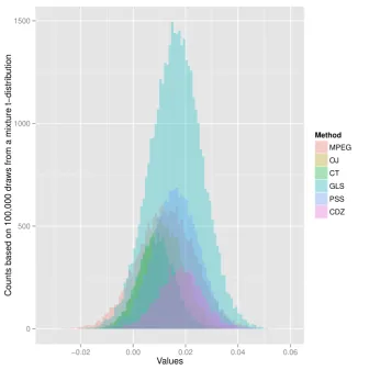
Figure 2 gives the answer to the question why model uncertainty does not affect the results. It shows the histogram for 100,000 draws from the mixture t-distribution of the MA1 approach. In particular, the histogram plots draws from the case in which the first difference of the value-weighted implied risk premium is regressed on the first difference of the variance (lower left block in Table 5). It becomes clear from this figure that all methods lead to very similar results, with only slight variation in the mean and the variance of the slope coefficient’s distribution. Not surprisingly, inferences based on a weighted average of similar distributions is similar to an inference based on any of these distributions.
In summary, this example shows that model averaging is an easy-to-use and flexible approach to incorporate model uncertainty. The results can be presented in a more concise way than based on separate evidence for each of the meth-ods. It is also straightforward to extend this approach to more specifications of a specific proxy class or even across proxy classes. It also emphasizes that alternative expected return proxies have their merits over realized returns. In cases in which reasonable alterations of an expected return proxy lead to similar conclusions, model uncertainty has a negligible effect on the results. However, it is vital to check this, as the next example shows.
4.4
The importance of cash flow (CF) and discount rate
(DR) news
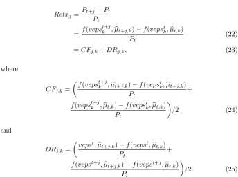
In a recent study, Chen et al. (2013) entertain the ICC to determine whether stock prices move because of revisions in expected cash flows or discount rates. Other studies predominantly entertain a vector-autoregressive (VAR) approach to estimate the time-series of expected returns and back out cash flow news as the residual. Instead, Chen et al. (2013) use direct expected cash flow measures, namely analyst forecasts. They show that capital gain returnsRetxbetweent+j andtcan be separated into two parts. First, a cash flow partCFj,k, which is the
part that explains changes in stock prices due to changes in analyst forecasts between t+j and t, holding the discount rate constant. Second, a discount rate part DFj,k, which is the part that explains changes in stock prices due to
changes in discount rates, holding the cash flows constant. As the subscript k indicates, both parts are dependent on the specific ICC method. In their paper, they estimate the discount rates with the CDZ method.
Concretely, recall from equation (19) and its derivatives that the stock price can be expressed as a function of the vector of future expected earningsvepst
k
then be expressed as:
Retxj= Pt
+j−Pt
Pt
= f(veps
t+j
k ,µbt+j,k)−f(vepstk,µbt,k)
Pt
(22)
=CFj,k+DRj,k, (23)
where
CFj,k=
f(vepst+j
k ,µbt+j,k)−f(vepstk,bµt+j,k)
Pt +
f(vepstk+j,µbt,k)−f(vepstk,bµt,k)
Pt
/2 (24)
and
DRj,k=
vepst,µb
t+j,k)−f(vepst,µbt,k)
Pt
+
f(vepst+j, b
µt+j,k)−f(vepst+j,µbt,k)
Pt
/2. (25)
The slope coefficients obtained from regressing CFj,k and DRj,k, respectively,
onRetxj represent the portion of capital gain returns driven by CF news and
DR news.
[image:26.595.124.469.141.397.2][Table 6 about here.]
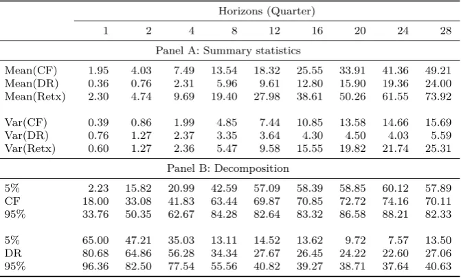
Table 6 is a replication of Table 2 in Chen et al. (2013) for the aggregate market.26 Although I use a different sample – for instance, I require that for every observation all ICCs are available –, the results are very similar. In both samples, the variation in capital gain returns is mostly explained by the DR news part for shorter horizons and by the CF news part for longer horizons. At a quarterly horizon, only 18%/16% of the return variation of the market portfolio is explained by CF news in my/their sample. This fraction increases to 70%/59% at a seven-year horizon. Also, the results are robust: at twelve quarters and beyond, the fraction of CF news is above 50%, even for the 5% percentile. In summary, these results imply that cash flow news is important in driving the stock price movements, based on evidence of the CDZ methods.
[Figure 3 about here.]
Do these results also hold if we incorporate model uncertainty into the anal-ysis? The short answer is no and Figure 3 shows why. It plots the fraction of the variation in Retx that is explained by CF news over various horizons and for different ICC methods. As becomes apparent, the view that most of the variation in capital gain returns is driven by CF news is only supported by the CDZ method and, to a lesser extent, by the CT method. All other methods come to the conclusion that DR news, even for longer horizons, is more im-portant. However, there is a very large variation across the different methods, which means that the return decomposition approach based on ICCs is very sensitive to the specific discount model.
The rationale behind this finding is that every ICC method equates the current stock price with a transformation of discounted expected dividends. Differences arise on how the second part is transformed. In this particular research question, the assumptions made here have a very large impact. Chen et al. (2013) assume that the earnings growth rate converges to the industry long-term growth rate provided by analysts over the next 15 years, although these growth rates are commonly interpreted to represent the next five years (see Claus and Thomas 2001) and are probably affected by analyst bias. Obviously, these growth assumptions are very sensitive to the current market environment. For example, during the dot-com bubble in 2001 the mean across the industry growth rates within my sample was as high as 25%. Assuming that investors expected earnings growth rates to converge to these growth rates for the next 15 years will obviously explain almost all of the capital gains that accrued over this period. Such an extreme assumption is not made by the other methods. For example, the PSS method assumes that the earnings growth rate in period 3 is the earnings growth rate provided by analysts and extrapolates this growth rate over 15 years to the historical average of the nominal GDP growth rate. This much more conservative assumption about expected earnings leaves a much larger part of capital gains unexplained and the ICC has to step in to fill the gap. The other extreme is the traditional GLS method, which anchors the current price on the very persistent current book value and the very persistent median ROE over the last decade to which ROEs for each firm are extrapolated from period 4 on. So the only parts left to explain price changes are the earnings forecasts of the first three years and the ICC. Hence, the latter has to account for a large part of the variation in returns, which actually results in a negative CF part for the GLS method in this sample.
method ignore the uncertainty we have about these assumptions. Since we al-ready know from Section 4.1 that the posterior model weights do not favor any ICC method unambiguously, it is obvious that the posterior distribution will be spread out. Nevertheless, it is instructive to apply the model averaging approach here.
First, I setφ to 1, which gives roughly equal weight to the evidence in the data and my prior beliefs that all ICC methods should be equally likely. The sampling from the parameter densities are done as in the previous example. That is, in the first case I sample from a mixture t-distribution, where each t-distribution’s parameters are estimated from an OLS with Newey-West cor-rected standard errors. In the second case, I apply a bootstrap approach in which I choose in each run an ICC method randomly, based on the posterior model weights, and obtain the regression coefficient for the specific bootstrap sample.
[Table 7 about here.]
Table 7 presents the results. As expected, incorporating model uncertainty widens the coverage regions considerably. Only for shorter horizons can one be reasonably sure that returns are mostly driven by DR news. For longer horizons, the intervals become too large to draw any reasonable conclusions. The results also show that the two approaches of model averaging yield similar results here.
5
Conclusion and Outlook
In this paper, I incorporate model uncertainty into the statistical inference that is based on expected return proxies. In the theoretical part, I show how results can be biased if one ignores the uncertainty in the selection process of such proxies and propose a model averaging approach that incorporates it. In the empirical part, I apply this approach to three research questions that are based on the implied cost of capital approach.
My main findings are that ignoring model uncertainty can overestimate the confidence of the results considerably. Hence, many apparently significant re-sults between expected return proxies and a variable of interest found in the literature could be due to ignoring both the performance evaluation of such a proxy and the uncertainty about this evaluation. Therefore, it should be an interesting endeavor to replicate previous studies with my model averaging ap-proach. In particular, it would be interesting to apply this approach to studies that look at the cross-section of expected returns.
alter-native specifications. This is in contrast with many studies in the ICC literature that focus only on one transformation of the dividend discount model and make minor adjustments to this model. If only proxies are considered that are virtu-ally identical, it is obvious that the results across these proxies will not uncover model uncertainty. Second, a researcher must be explicit about any prior be-liefs made about the quality of the proxies. In current studies, it is common practice to implicitly set the prior weight on one proxy to one and to ignore the evidence of other reasonable specifications, at least for the main part of the em-pirical analysis. This approach is unsatisfying for two reasons: First, it ignores evidence about the performance of each proxy to explain subsequent realized returns, which each proxy has to explain eventually. Second, it conceals the uncertainty inherent in the proxy selection process.
The model averaging approach inherits its weaknesses from the underlying proxies. If all proxies are systematically biased, the results based on evidence across these models will also be biased. If a specification is favored by the inclusion of many minor variations of this specification, the posterior results will also put too much emphasizes on this specification. If shocks on subsequent realized returns are correlated with a specific ICC method in sample, predictive regressions will unjustly favor it over other methods and results will be biased towards this method.
In summary, my results provide evidence that model uncertainty in alter-native expected return proxies is the complement of parameter uncertainty in realized returns. My study is a first attempt to answer the question which of those is more worrisome for the applied researcher.
References
Avramov, Doron. 2002. Stock return predictability and model uncertainty. Jour-nal of Financial Economics64 (3): 423–458.
Binsbergen, Jules van, Wouter Hueskes, Ralph Koijen, and Evert Vrugt. 2013. Equity yields.Journal of Financial Economics Forthcoming.
Campello, Murillo, Long Chen, and Lu Zhang. 2008. Expected returns, yield spreads, and asset pricing tests. Review of Financial Studies21 (3): 1297– 1338.
Chen, Long, Zhi Da, and Xinlei Zhao. 2013. What drives stock price movements?
Review of Financial Studies26 (4): 841–876.
Claeskens, Gerda, and Nils Lid Hjort. 2008.Model selection and model averaging.
Claus, James, and Jacob Thomas. 2001. Equity premia as low as three percent? evidence from analysts’ earnings forecasts for domestic and international stock markets. The Journal of Finance56 (5): 1629–1666.
Cochrane, John H. 2011. Presidential address: discount rates. The Journal of Finance66 (4): 1047–1108.
Cremers, Martijn. 2002. Stock return predictability: a bayesian model selection perspective.Review of Financial Studies 15 (4): 1223–1249.
Draper, David. 1995. Assessment and propagation of model uncertainty.Journal of the Royal Statistical Society. Series B (Methodological):45–97.
Easton, Peter. 2004. PE ratios, PEG ratios, and estimating the implied expected rate of return on equity capital.The Accounting Review79 (1): 73–95.
———. 2007. Estimating the cost of capital implied by market prices and ac-counting data.Foundations and Trends® in Accounting 2 (4): 241–364.
Easton, Peter, and Steven Monahan. 2005. An evaluation of accounting-based measures of expected returns.The Accounting Review 80 (2): 501–538.
Elton, Edwin. 1999. Presidential address: expected return, realized return, and asset pricing tests.The Journal of Finance54 (4): 1199–1220.
Fama, Eugene, and Kenneth French. 1997. Industry costs of equity.Journal of Financial Economics43 (2): 153–193.
———. 2002. The equity premium.The Journal of Finance 57 (2): 637–659.
Fernandez, Carmen, Eduardo Ley, and Mark Steel. 2001. Model uncertainty in cross-country growth regressions.Journal of Applied Econometrics16 (5): 563–576.
Friewald, Nils, Christian Wagner, and Josef Zechner. 2013. The cross-section of credit risk premia and equity returns.The Journal of FinanceForthcoming.
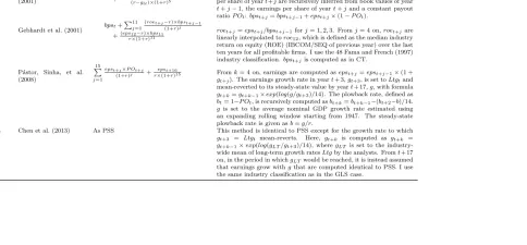
Gebhardt, William, Charles Lee, and Bhaskaran Swaminathan. 2001. Toward an implied cost of capital.Journal of Accounting Research39 (1): 135–176.
Gode, Dan, and Partha Mohanram. 2003. Inferring the cost of capital using the Ohlson–Juettner model.Review of Accounting Studies8 (4): 399–431.
Guay, Wayne, SP Kothari, and Susan Shu. 2011. Properties of implied cost of capital using analysts’ forecasts.Australian Journal of Management36 (2): 125–149.
Hail, Luzi, and Christian Leuz. 2009. Cost of capital effects and changes in growth expectations around us cross-listings. Journal of Financial Eco-nomics93 (3): 428–454.
Hou, Kewei, Mathijs van Dijk, and Yinglei Zhang. 2012. The implied cost of capital: a new approach. Journal of Accounting and Economics 53 (3): 504–526.
Hughes, John, Jing Liu, and Jun Liu. 2009. On the relation between expected returns and implied cost of capital.Review of Accounting Studies14 (2-3): 246–259.
Kass, Robert, and Adrian Raftery. 1995. Bayes factors.Journal of the American Statistical Association 90 (430): 773–795.
Koijen, Ralph, and Stijn Van Nieuwerburgh. 2011. Predictability of returns and cash flows. Annual Review of Financial Economics3:467–491.
Leamer, Edward. 1978.Specification searches: ad hoc inference with nonexperi-mental data.Wiley New York.
Lee, Charles, David Ng, and Bhaskaran Swaminathan. 2009. Testing interna-tional asset pricing models using implied costs of capital.Journal of Finan-cial and Quantitative Analysis44 (2): 307–335.
Lee, Charles, Eric So, and Charles Wang. 2011. Evaluating implied cost of cap-ital estimates. Working Paper.
Ley, Eduardo, and Mark Steel. 2009. On the effect of prior assumptions in bayesian model averaging with applications to growth regression. Journal of Applied Econometrics24 (4): 651–674.
Li, Yan, David Ng, and Bhaskaran Swaminathan. 2013. Predicting market re-turns using aggregate implied cost of capital. Journal of Financial Eco-nomicsForthcoming.
Lundblad, Christian. 2007. The risk return tradeoff in the long run: 1836–2003.
Journal of Financial Economics 85 (1): 123–150.
P´astor, ˇLuboˇs, Meenakshi Sinha, and Bhaskaran Swaminathan. 2008. Estimat-ing the intertemporal risk–return tradeoff usEstimat-ing the implied cost of capital.
The Journal of Finance63 (6): 2859–2897.
P´astor, ˇLuboˇs, and Robert Stambaugh. 2009. Predictive systems: living with imperfect predictors.The Journal of Finance64 (4): 1583–1628.
Ramnath, Sundaresh, Steve Rock, and Philip Shane. 2008. The financial analyst forecasting literature: a taxonomy with suggestions for further research.
International Journal of Forecasting 24 (1): 34–75.
Sadka, Gil, and Ronnie Sadka. 2009. Predictability and the earnings–returns relation.Journal of Financial Economics 94 (1): 87–106.
Sala-I-Martin, Xavier, Gernot Doppelhofer, and Ronald Miller. 2004. Deter-minants of long-term growth: a bayesian averaging of classical estimates (BACE) approach.American Economic Review94 (4): 813–835.
Wright, Jonathan. 2008. Bayesian model averaging and exchange rate forecasts.
Journal of Econometrics 146 (2): 329–341.