Munich Personal RePEc Archive
Continuous invertibility and stable QML
estimation of the EGARCH(1,1) model
Wintenberger, Olivier
7 January 2013
Online at
https://mpra.ub.uni-muenchen.de/46027/
EGARCH(1,1) MODEL
OLIVIER WINTENBERGER
Abstract. We introduce the notion of continuous invertibility on a compact set for volatility models driven by a Stochastic Recurrence Equation (SRE). We prove the strong consistency of the Quasi Maximum Likelihood Estimator (QMLE) when the optimization procedure is done on a continuously invertible domain. This approach gives for the first time the strong consistency of the QMLE used by Nelson in [29] for the EGARCH(1,1) model under explicit but non observable conditions. In practice, we propose to stabilize the QMLE by constraining the optimization procedure to an empirical continuously invertible domain. The new method, called Stable QMLE (SQMLE), is strongly consistent when the observations follow an invertible EGARCH(1,1) model. We also give the asymptotic normality of the SQMLE under additional minimal assumptions.
AMS 2000 subject classifications: Primary 62F12; Secondary 60H25, 62F10, 62M20, 62M10, 91B84.
Keywords and phrases: Invertible models, volatility models, quasi maximum likelihood, strong consistency, asymptotic normality, exponential GARCH, stochastic recurrence equation.
1. Introduction
Since the seminal papers [14, 7], the General Autoregressive Conditional Heteroskedasticity (GARCH) type models have been successfully applied to financial time series modeling. One of the stylized facts observed on the data is the asymmetry with respect to (wrt) shocks [11]: a neg-ative past observation impacts the present volatility more importantly than a positive one. Nelson introduced in [29] the Exponential-GARCH (EGARCH) model that reproduces this asymmetric effect. Not surprisingly, theoretical investigations of EGARCH has attracted lot of attention since then, see for example [20, 27]. However, the properties of the Quasi Maximum Likelihood Estimator (QMLE) used empirically in [29] was not proved except in some degenerate case, see [34]. We give in this paper some sufficient conditions for the strong consistency and the asymptotic normality of the QMLE in the EGARCH(1,1) model. Our approach of the strong consistency is based on the natural notion of continuous invertibility that we introduce in the general setting of volatility model solutions of a Stochastic Recurrent Equation (SRE).
Consider a real valued volatility model of the form Xt = σtZt where σt is the volatility and
where the innovations Zt are normalized, centered independent identical distributed (iid) random
vectors. It is assumed that a transformation of the volatility satisfies some parametric SRE (also called Iterated Random Function): there exist a functionh and some ψt measurable wrt Zt such
that the following relations
(1) h(σ2t+1) =ψt(h(σ2t), θ0), ∀t∈Z
hold. Classical examples are the GARCH(1,1) and EGARCH(1,1) models:
GARCH(1,1): σ2
t+1=α0+β0σt2+γ0Xt2,
(2)
EGARCH(1,1): log(σ2
t+1) =α0+β0log(σt2) + (γ0Zt+δ0|Zt|).
(3)
In practice, the innovationsZtare not observed. WritingZt=Xt/σtin the expression ofψtwrt
Zt, we invert the model, i.e we consider a new SRE driven by a functionφtof the observationXt,
(4) h(σt2+1) =φt(h(σt2), θ0), t∈Z.
For instance, we obtain from (2) the inverted modelφt(x, θ) =α+βx+γXt2 for the GARCH(1,1)
model. For the EGARCH(1,1) model, we obtain from (3) the inverted model (5) φt(x, θ) =α+βx+ (γXt+δ|Xt|) exp(−x/2).
In accordance with the notions of invertibility given in [18, 36, 33, 34], we will say that the model is invertible if the SRE (4) is stable. Then, as the functionsφtare observed, the volatility is efficiently
forecasted by using recursively the relation
(6) ht+1=φt(ht, θ0), t≥0,
from an arbitrary initial value h0. Sufficient conditions for the convergence of this SRE are the
negativity of a Lyapunov coefficient and the existence of logarithmic moments, see [8]. So the GARCH(1,1) model is invertible as soon as 0 ≤ β0 < 1. The invertibility of the EGARCH(1,1)
model is more complicated to assert due to the exponential function in (5). The recursive relation on ht+1 can explode to −∞ for small negative values ofht and negative values of γ0Xt+δ0|Xt|.
However, assuming that δ0 ≥ |γ0|, the relationγ0Xt+δ0|Xt| >0 holds and conditions for
invert-ibility of the EGARCH(1,1), denoted hereafter INV(θ0), are obtained in [33, 34]:
INV(θ0): δ0≥ |γ0|and
(7) E[log(max{β0,2−1(γ
0X0+δ0|X0|) exp(−2−1α0/(1−β0))−β0})]<0.
On the oppposite, Sorokin introduces in [32] sufficient conditions onθ0for the EGARCH(1,1) model
to be non-invertible. Then the SRE (5) is completely chaotic for any possible choice of the initial valueh0 and the volatility forecasting procedure based on the model (4) is not reliable.
In practice, the valueθ0= (α0, β0, γ0, δ0) of the Data Generating Process (DGP) EGARCH(1,1)
is unknown. Nelson proposed in [29] to estimateθ0with the Quasi Maximum Likelihood Estimator
(QMLE). Let us recall the definition of this classical estimator that estimates efficiently many GARCH models, see [5] for the GARCH case and [16] for the ARMA-GARCH case. To construct the QMLE one approximates the volatility using the observed SRE (6) at anyθ. Assume that the SREs driven byφt(·, θ) are stable for anyθ. Let us consider the functions ˆgt(θ) defined for anyθas
the recursive solutions of the SRE
(8) gˆt+1(θ) =φt(ˆgt(θ), θ), t≥0,
for some arbitrary initial value ˆg0(θ). Assume thathis a bijective function of inverseℓ >0. Then
ℓ(ˆgt(θ0)) has a limiting law that coincides with the one ofσ2t. The Quasi Likelihood (QL) criteria
is defined as
(9) 2nLˆn(θ) = n
X
t=1
ˆ
lt(θ) = n
X
t=1
Xt2/ℓ(ˆgt(θ))2+ log(ℓ(ˆgt(θ)).
The associatedM-estimator is the QMLE ˆθn defined by optimizing the QL on some compact set Θ
ˆ
θn= argminθ∈ΘLˆn(θ).
This estimator has been used since the seminal paper of Nelson [29] for estimating the EGARCH(1,1) model without any theoretical justification, see for example [10]. The inverted EGARCH(1,1) model is driven by the SRE (8) that expresses as (denotingℓ(ˆgt) = ˆσt2)
The consistency and the asymptotic normality are not proved except in the degenerate case β= 0 for all θ ∈ Θ in [33]. The problem of the procedure (and of any volatility forecast) is that the inverted EGARCH(1,1) model (10) is stable only for some values of θ. Thus, contrary to other GARCH models, the QML estimation procedure is not always reliable for the EGARCH model, see the discussion in [19]. Thus, other estimation procedure has been investigated such as the bayesian, bias correction and the Whittle procedure in [38, 12, 39] respectively. Another approach is to in-troduce models that behave like the EGARCH(1,1) model but where the QMLE could be more reliable, see [19, 35, 15].
We prove the strong consistency of the QMLE for the general model (1) when the maximization procedure is done on a continuously invertible domain. We give sufficient conditions called the continuous invertibility of the model such that the QMLE is strongly consistent. More precisely we assume that the SRE (8) produces continuous functions ˆgt ofθ on Θ. The continuous invertibility
holds when the limiting law of ˆgt corresponds to the law of some continuous functiongton Θ that
does not depend on the initial function ˆg0. The continuous invertibility ensures the stability of the
estimation procedure regardless the initial function ˆg0 chosen arbitrarily in practice. Under few
other assumptions, we prove that the QMLE is strongly consistent for continuously invertible mod-els on the compact set Θ. The continuous invertiblity should be checked systematically on modmod-els before using QMLE. One example of such continuously invertible models with properties similar than the EGARCH model is the Log-GARCH model studied in [15].
As the continuous invertibility is an abstract assumption, we provide sufficient conditions for continuous invertibility collected in the assumption (CI) below. These conditions ensure the in-vertibility of the model at any pointθof the compact set Θ and some regularity of the model with respect to the parameterθ. As the inverted EGARCH(1,1) model (10) is a regular function ofθ, it satisfies(CI)on any Θ such that the invertibility condition INV(θ) is satisfied for anyθ∈Θ. Thus we prove the strong consistency of the QMLE for the invertible EGARCH(1,1) model when INV(θ) is satisfied for anyθ∈Θ. It is a serious advantage of our approach based on the continuous invert-ibility condition(CI)compared with the approach of [33]. Based on uniform Lipschitz coefficients this last approach is more restrictive than our when applied to the EGARCH(1,1) model. Moreover, we also prove the strong consistency of the natural volatility forecasting ˆσ2
n = ℓ(ˆgn(ˆθn)) of σ2n+1
under(CI). Continuous invertibility seems to be well suited to assert volatility forecasting because ˆ
σ2
n expresses as functions ˆgn evaluated at points ˆθn 6=θ0. To infer in practice the EGARCH(1,1)
model, we propose to stabilize the QMLE. We constrain the QMLE on some compact set satisfy-ing the empirical version of the condition INV(θ0). This new estimator ˆθSn called Stable QMLE
(SQMLE) produces only reliable volatility forecasting such that ˆσ2
n =ℓ(ˆgn(ˆθnS)) does not depend
asymptotically of the initial value ˆσ2
0=ℓ(ˆg0). It is not the case of the classical QMLE the continuous
invertibility conditionIN V(θ) is not observed in practice. Thus INV(θ) might not be satisfied for any θ in the compact set Θ of the maximization procedure. And the whole procedure might have some chaotic behavior with respect to any initial value ˆσ2
0 used in the inverted model.
We consider conditions of moments(MM)only at the pointθ0where the expression of the score
vec-tor simplifies. In the EGARCH(1,1) model, the conditions(MM)take the simple formE[Z4
0]<∞
andE[(β0−2−1(γ
0Z0+δ0|Z0|)2]<1 and can be checked in practice by estimating the innovations.
We believe that this new approach gives sharp conditions for asymptotic normality for other models.
The paper is organized as follows. In Section 2, we discuss the standard notions of invertibility and introduce the continuous invertibility and its sufficient condition (CI). We prove the strong consistency of the QMLE for general continuously invertible models in Section 4.1. The consistency of the volatility forecasting is also proved under the sufficient condition(CI). We apply this results in the EGARCH(1,1) model in Section 4. For this model, we propose a new method called Stable QMLE that produces only reliable volatility forecasting. The asymptotic normality of SQMLE for the EGARCH(1,1) model is given in Section 5. The proofs of technical Lemmas are collected in Section 6.
2. Preliminaries
2.1. The general volatility model. In this paper, the innovationsZt∈Rare iid random variables
(r.v.) such thatZt is centered and normalized, i.e. E[Z0] = 0 and E[Z02] = 1. Consider the general
DGPXt=σtZt satisfyingh(σt2+1) =ψt(h(σ2t), θ0) for allt∈Z. The functionhis a bijection from
some subsetR+to some subset ofRof inverseℓcalled the link function. A first question regarding
such general SRE is the existence of the model, i.e. wether or not a stationary solution exists. Hereafter, we work under the general assumption
(ST): The SRE (1) admits a unique stationary solution denoted (σ2
t) that is non anticipative,
i.e. σ2
t is independent of (Zt, Zt+1, Zt+2, . . .) for all t ∈ Z, and has finite log-moments:
Elog+σ2 0<∞.
The GARCH(1,1) model (2) satisfies the condition(ST)if and only if (iff)E[log(β0+γ0Z2 0)]<0,
see [28] for the existence of the stationary solution and [5] for the existence of log moments. The EGARCH(1,1) model (3) satisfies the condition(ST)iff|β0|<1, see [29]. In this case, the model
has nice ergodic properties: any process recursively defined by the SRE from an arbitrary initial value approximates exponentially fast a.s. the original process (σ2
t). In the sequel, we say that
the sequence of non negative r.v. (Wt) converges exponentially almost surely to 0, Wt e.a.s.
−−−→0 as
t→ ∞, ifWt=o(e−Ct) a.s. for some r.v. C >0. We will also use the notationx+ for the positive
part ofx, i.e. x+=x
∨0 for anyx∈R.
2.2. Invertible models. Under (ST) the process (Xt) is stationary, non anticipative and thus
ergodic as a Bernoulli shift of an ergodic sequence (Zt), see [24]. Let us now investigate the question
of invertibility of the general model (1). The classical notions of invertibility are related with convergences of SRE and thus are implied by Lyapunov conditions of Theorem 3.1 in [8]. Following [36], we say that a volatility model is invertible if the volatility can be expressed as a function of the past observed values:
Definition 1. Under(ST), the model is invertible if the sequence of the volatilities(σ2
t)is adapted
to the filtration generated by (Xt−1, Xt−2,· · ·).
Using the relation Zt=Xt/ℓ(h(σt)) in the expression of ψt yields the new SRE (4): h(σt2+1) =
φt(h(σ2t), θ0). Now the random functions φt(·, θ0) depends only on Xt. As (Xt) is an ergodic
and stationary process, it is also the case of the sequence of parametrized maps (φt(·, θ0)). Using
there exists r >0 satisfying (11)
inv(θ0)E[log+|φ0(x, θ0)|]<∞for somex∈E, E[log+Λ(φ0(·, θ0))]<∞andE[log Λ(φ0(·, θ0)(r))]<0.
Here Λ(f) denotes the Lipschitz coefficient of any function f defined by the relation (in the case wheref is real valued)
Λ(f) = sup
x6=y
|f(x)−f(y)|
|x−y|
ft(r) denotes the iterate fto ft−1o· · ·o ft−r for any sequence of function (ft). The conditions (11)
are called the conditions of invertibility in [34] and is proved there that
Proposition 1. Under(ST) and (11), the general model (4) is invertible. The GARCH(1,1) model (2) is invertible as soon as 0≤β0<1.
The invertibility of the EGARCH(1,1) model is more difficult to assert due to the exponential function in the SRE (5). Let us describe the sufficient condition of invertibility INV(θ0) of the
EGARCH(1,1) model given in [33, 34]. It expresses as a Lyapunov condition (7) on the coefficients
θ0= (α0, β0, γ0, δ0). This condition does not depend onα0when the DGP (Xt) is itself the stationary
solution of the EGARCH(1,1) model forθ0. Indeed, (logσt2) admits a MA(∞) representation
logσ2t =α0(1−β0)−1+ ∞
X
k=1
β0k−1(γ0Zt−k+δ0|Zt−k|).
Plugging in this MA(∞) representation into (7), we obtain the equivalent sufficient condition
(12) Ehlogmaxnβ0,2−1exp2−1 ∞
X
k=0
βk
0(γ0Z−k−1+δ0|Z−k−1|)
(γ0Z0+δ0|Z0|)−β0
oi
<0.
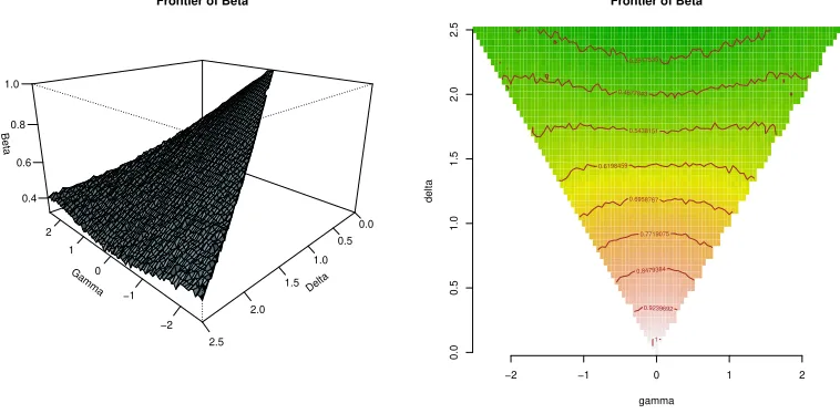
Using the Monte Carlo algorithm and assuming thatZ0 isN(0,1)-distributed, we report in Figure
1 the largest values ofβ0 that satisfies the condition (7) on a grid of values of (γ0, δ0).
Gamma
−2 −1 0 1 2
Delta
0.0 0.5 1.0
1.5
2.0
2.5
Beta
0.4 0.6 0.8 1.0
Frontier of Beta
gamma
delta
0.3917535
0.4677843
0.5438151
0.6198459
0.6958767
0.7719075
0.8479384
0.9239692
1
−2 −1 0 1 2
0.0
0.5
1.0
1.5
2.0
2.5
[image:6.612.118.497.482.669.2]Frontier of Beta
The constraint onβ0is always stronger than the stationary constraint|β0|<1. It exists
station-ary EGARCH(1,1) models that are not invertible, i.e. the inverted model
log ˆσt2+1=α0+β0logσt2+ (γ0Xt+δ0|Xt|) exp(−logσt2+1/2), t≥0,
is not stable wrt any possible choice of initial value log ˆσ2
0. On the opposite, Sorokin exhibits in [32]
sufficient conditions for some chaotic behaviour of the inverted EGARCH(1,1) model under|β0|<1.
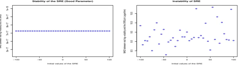
To emphasize the danger to work with non invertible EGARCH(1,1) models, we report in Figure 2 the convergence criterionPN
t=1(logσt2−log ˆσ2t) wrt arbitrary initial values for two different values
of θ0 (N = 10 000). The first picture represents a stable case where INV(θ0) holds. The second
picture represents a chaotic case where the condition of non invertibility given in [32] is satisfied. The stationary constraint |β0| < 1 is satisfied in both cases. It is interesting to note that the
convergence criterion does not explode in the chaotic case. It is an important difference between the non invertible GARCH(1,1) and EGARCH(1,1) models: the non invertible GARCH(1,1) is always explosive because it is also non stationary. The inference by QMLE remains stable due to this very specific behaviour, see [22]. On the opposite, we have driven numerical experiments and we are convinced that the QMLE procedure is not stable when the EGARCH(1,1) model is non invertible. It is not surprising as it is not possible to recover the volatility process from the inverted model, even when the parameterθ0 of the DGP is known.
● ● ● ● ● ● ● ● ● ● ● ● ● ● ● ● ● ● ● ● ● ● ● ● ● ● ● ● ● ● ● ● ● ● ● ● ● ● ● ● ●
−100 −50 0 50 100
5e−17 6e−17 7e−17 8e−17 9e−17 1e−16
Stability of the SRE (Good Parameter)
Initial values of the SRE
MAD betw
een real log−v
olatility and the SREs
● ● ● ● ● ● ● ● ● ● ● ● ● ● ● ● ● ● ● ● ● ● ● ● ● ● ● ● ● ● ● ● ● ● ● ● ● ● ● ● ●
−100 −50 0 50 100
8.5
9.0
9.5
10.0
10.5
Instablilty of SRE
Initial values of the SRE
MAD betw
een real log−v
olatility and the SREs(in Logar
[image:7.612.109.497.357.466.2]ithm)
Figure 2. Stable and non stable inverted EGARCH(1,1) models.
3. Strong consistency of the QMLE on continuously invertible domains
3.1. Continuously invertible models. Assume now that the DGP follows the general model (4) for an unknown valueθ0. Consider the inference of the QMLE ˆθn defined as ˆθn= argminθ∈ΘLˆn(θ)
for some compact set Θ. Here ˆLn is the QL criteria defined in (9) and based on the approximation
ˆ
gt(θ) of the volatility:
ˆ
gt+1(θ) =φt(ˆgt(θ), θ), ∀t≥0,∀θ∈Θ
starting at an arbitrary initial value ˆg0(θ), for any θ ∈ Θ. The invertibility of the model is not
sufficient to assert the consistency of the inference: as the parameterθ0is unknown, the conditions
of invertibility (11) do not provide the stability of the approximation ˆgt(θ) wrt the initial value ˆg0(θ)
when θ 6=θ0. satisfied for (φt(·, θ)) for any θ ∈Θ then the unique stationary solution (gt) exists
and is defined by the relation
(13) gt+1(θ) =φt(gt(θ), θ), ∀t∈Z,∀θ∈Θ.
Assume there exists some subsetK ofRsuch that the random functions (x, θ)→φt(x, θ) restricted
function on Θ that takes its values in K. Denote k · kΘ the uniform norm and CΘ the space of
continuous functions from Θ toK. By a recursive argument, it is obvious that the random functions ˆ
gtbelong toCΘ for allt≥0.
We are now ready to define the notion of continuous invertibility:
Definition 2. The model is continuously invertible onΘiffkˆgt(θ)−gt(θ)kΘ→0a.s. whent→ ∞.
This continuous invertibility notion is crucial for the strong consistency of the QMLE.
3.2. Strong consistency of the QMLE constrained to a continuously invertible domain.
Let us assume the regularity and boundedness from below on the link functionℓ:
(LB): The mapsx→1/ℓ(x) and log(ℓ(x)) are Lipschitz functions onKand there existsm >0 such thatℓ(x)≥mfor allx∈ K.
Classically, we also assume the identifiability of the model
(ID): ℓ(g0(θ)) =σ02 a.s. for someθ∈Θ iff θ=θ0.
The consistency of the QMLE follows from the continuous invertibility notion:
Theorem 1. Assume that (ST),(LB)and(ID)for a volatility model that is continuously invertible on the compact setΘ. Then the QMLE onΘis strongly consistent,θˆn→θ0 a.s., whenθ0∈Θ.
Proof. First, note that from the continuous invertibility of the model on Θ, the SRE (13) admits a stationary solution inE=CΘ that is a separable complete metric space (equipped with the metric
d(x, y) =kx−ykΘ). Let us denote Φt the mapping acting onCΘ and satisfying
gt+1= Φt(gt) iff gt+1(θ) =φt(gt(θ), θ), ∀θ∈Θ.
We will apply the principle of Letac [25] extended to the stationary sequences as in [34]: the existence of a unique stationary non anticipative solution follows from the convergence a.s. of the backward equation for any initial valueg∈ CΘ:
Zt(g) := Φ0oΦ−1o· · ·oΦ−t(g)→t→∞Z
where Z does not depend on g. By stationarity,Zt(g) is distributed as ˆgt when ˆg0=g. Thus, we
have
P( lim
t→∞kZt(g)−g0kΘ= 0) =
P( lim
t→∞kgˆt−gtkΘ= 0)
whereg0(θ) is well defined for eachθ∈Θ as the solution of the SRE (13). Thus, under continuous
invertibility, an application of Letac’s principle leads to the existence of a unique stationary solution distributed denoted also (gt) that coincides withgt(θ) at any pointθ∈Θ. In particular,gtbelongs
toCΘ and
2nLn(θ) = n
X
t=1
lt(θ) = n
X
t=1
Xt2/ℓ(gt(θ))2+ log(ℓ(gt(θ)).
is a continuous function on Θ.
Let us turn to the proof of the strong consistency based on standard arguments, see for example the book of Francq and Zako¨ıan [17]. As the model satisfies the identifiability condition(ID), the strong consistency follows the intermediate results
(a) limn→∞supθ∈Θ|Ln(θ)−Lˆn(θ)|= 0 a.s.
(b) E|l0(θ0)|<∞and ifθ6=θ0thenE[l0(θ)]>E[l0(θ0)].
(c) Anyθ6=θ0 has a neighborhoodV(θ) such that
lim inf
n→∞θ∗∈infV(θ)
ˆ
Let us prove that (a) is satisfied when the model is continuously invertible and the condition
(LB)holds. As 1/ℓand log(ℓ) are Lipschitz continuous functions there exists some constantC >0 such that
(14) |Ln(θ)−Lˆn(θ)| ≤C
1
n
n
X
t=1
|gˆt(θ)−gt(θ)|.
The desired convergence to 0 of the upper bound that is a Cesaro mean follows from the definition of the continuous invertibility.
The first assertion of (b) follows from the identity
l0(θ0) = log(σ02) +Z02.
Thus, asσ0=ℓ(g0(θ0))≥mfrom(LB)andElog+σ20<∞under(ST), we have that log(σ20) is
in-tegrable. Moreover,EZ2
0 = 1 by assumption and the assertionE|l0(θ0)|<∞is proved. To prove the
second assertion, note thatθ→E[l0(θ)] has a unique minimum iff E[σ2
0/ℓ(g0(θ))−log(σ02/ℓ(g0(θ))]
has a unique minimum. Under the identifiability condition, as x−log(x)≥ 1 for all x > 0 with equality iffx= 1, we deduce that for anyθ6=θ0 we have E[l0(θ)]>E[l0(θ0)].
Finally, let us prove (c) under continuous invertibility, (LB)and(ID). First, under continuous invertibility, we have
lim inf
θ∗→θ
ˆ
Ln(θ∗) = lim inf
n→∞θ∗∈infV(θ)Ln(θ
∗) + lim inf
n→∞θ∗∈infV(θ)( ˆLn(θ
∗)
−Ln(θ∗))
= lim inf
n→∞θ∗∈infV(θ)Ln(θ
∗)
by using the convergence to 0 of the Cesaro mean (14). Second, by ergodicity of the stationary solution (gt) we have the ergodicity of the sequence (infθ∗∈V(θ)lt(θ∗)). Moreover, under the condition
(LB), we have that infθ∗∈V(θ)lt(θ∗) ≥ log(m) > −∞ a.s. Then, for any K > 0, the sequence
infθ∗∈V(θ)lt(θ∗)∧K is integrable. We use the classical SLLN and obtain
lim
n→∞θ∗∈infV(θ)Ln(θ
∗)
∧K=Eh inf
θ∗∈V(θ)l0(θ
∗)
∧Ki a.s.
LettingK→ −∞we obtain that
lim
n→∞θ∗∈infV(θ)Ln(θ
∗) =Eh inf
θ∗∈V(θ)l0(θ
∗)i
∈R∪ {+∞}.
Finally, remark that by continuity ofθ→gt(θ) the functionl0 is continuous. Thus, for anyε > 0
we can find a neighborhoodV(θ) such that
Eh inf
θ∗∈V(θ)l0(θ
∗)i
≥E[l0(θ)] +ε.
From the second assertion of (b) we chooseε >0 such thatE[l0(θ)] +ε >E[l0(θ0)] and (c) is proved.
The end of the proof of the strong consistency is based on a classical compact argument and thus
is omitted.
Consider some generic functionf :K ×Θ7→ K. Assume that there exists a continuous function Λf on Θ such that for eachx,y∈E we have
|f(x, θ)−f(y, θ)| ≤Λf(θ)|x−y|.
The approach followed by Straumann and Mikosch in [34] is to consider the SRE (8) in the complete metric space of continuous functionsCΘ on Θ with values inK equipped withd(x, y) =kx−ykΘ.
Straightforward conditions for continuous invertibility are the following ones
(15) Elog+(kφ0(y,·)kΘ)<∞for some y∈ K, Elog+(kΛφ0kΘ)< ∞andElog Λ
φ(0r)
Θ
<0.
The EGARCH(1,1) model satisfies this condition under restrictive assumptions on Θ, for example whenβ= 0 for any θ∈Θ, see [33].
We collect more general sufficient conditions for continuous invertibility in the assumption(CI)
(CI): Elog+(kφ0(y,·)kΘ)<∞for somey∈ K,Elog+(kΛφ0kΘ)<∞andElog Λ
φ(0r)(θ)
<0 for anyθ∈Θ.
The difference with conditions (15) is that the Lyapunov condition holds pointwisely and not nec-essarily uniformly on Θ. Of course(CI) is weaker than the uniform Lyapunov condition (15). Due to the regularity of classical models wrt toθ,(CI)is satisfied as soon as the model is invertible on Θ (see Section 4.1 for the EGARCH(1,1) case). Next Theorem proves that the continuity argument is sufficient to assert continuous invertibility:
Theorem 2. If(ST)and(CI)hold on some compact setΘthen the model is continuously invertible onΘ.
Proof. For anyρ >0, let us write Λ(∗r)(θ, ρ) = sup{Λφ(r) 0 (θ
∗), θ∗∈B(θ, ρ)∩Θ}, whereB(θ, ρ) stands
for the closed ball centered atθwith radiusρ. Note that for anyK >0 we haveE[sup
Θ|log Λ (r)
φ0(θ)∨
K|] < ∞ because E[sup
Θlog+Λφ0(r)(θ)] < ∞ under (CI). Applying the dominated convergence
theorem we obtain limρ→0E[log Λ(∗r)(θ, ρ)∨K] = E[limρ→0log Λ(∗r)(θ, ρ)∨K]. By continuity we
have limρ→0log Λ(∗r)(θ, ρ) = log Λφ(r)
0 (θ) and for sufficiently smallK <0
lim
ρ→0
E[log Λ(∗r)(θ, ρ)∨K] =E[log Λ
φ(r)0 (θ)∨K]<0.
Thus, there exists anǫ >0 such that
E[log Λ(∗r)(θ, ǫ)]≤E[log Λ∗(r)(θ, ǫ)∨K]<0.
DenoteV(θ) the compact neighborhoodB(θ, ǫ)∩Θ ofθ. Let us now work onCV(θ), the complete
In this setting (ˆgt) satisfies a functional SRE ˆgt+1= Φt(ˆgt) with Lipschitz coefficients satisfying
Λ(Φ(tr))≤ sup
s1,s2∈C(V(θ))
kΦ(tr)(s1)−Φt(r)(s2)kV(θ)
ks1−s2kV(θ)
≤ sup
s1,s2∈C(V(θ))
supθ∗∈V(θ)kφ (r)
t (s1(θ∗), θ∗)−φt(r)(s2(θ∗), θ∗)k
ks1−s2kV(θ)
≤ sup
s1,s2∈C(V(θ))
supθ∗∈V(θ)Λ(φ (r)
t (·, θ∗))ks1(θ∗)−s2(θ∗)k
ks1−s2kV(θ)
≤ sup
s1,s2∈C(V(θ))
supθ∗∈V(θ)Λ(φ (r)
t (·, θ∗))ks1−s2kV(θ)
ks1−s2kV(θ) ≤
Λ(∗r)(θ, ǫ).
As E[log+(kΦ0(y)kV(θ))] ≤E[log+(kφ0(y, θ)kΘ)]<∞, E[log+(Λ(Φ0))]≤E[log+(kΛφ0(θ)kΘ)]<∞
under(CI)andE(log Λ(Φ(0r)))<0 we can apply Theorem 3.1 of [8]. The unique stationary solution
(gt) exists and satisfies
(16) kgˆt−gtkV(θ)
e.a.s.
−−−→0.
Now, let us remark that Θ =∪θ∈ΘV(θ). As Θ is a compact set, there exists a finite numberN such
that Θ =∪N
k=1V(θk) and we obtain
kgˆt−gtkV(θk)
e.a.s.
−−−→0 ∀1≤k≤N.
The desired result follows from the indentityk · kΘ=∨Nk=1k · kV(θk).
3.4. Volatility forecasting. Based on the QMLE ˆθn we deduce a natural forecasting ˆσn2+1 =
ℓ(ˆgn(ˆθn)) of the volatilityσn2+1. It is strongly consistent:
Theorem 3. Assume that(ST),(LB),(ID)and(CI)hold forθ0∈Θ. Then|σˆ2n+1−σn2+1|
a.s.
−−→0
asn→ ∞.
Proof. Theorems 1 and 2 assert the strong consistency of ˆθn under the assumption of Theorem 3.
By continuity ofℓand continuous invertibility on Θ,|ℓ(ˆgt(ˆθn))−ℓ(gt(ˆθn))|−−→a.s. 0. Thus, using again
the continuity ofℓ, the result is proved if|gt(ˆθn)−gt(θ0)|
a.s.
−−→0. Keeping the notation used in the proofs of Theorems 1 and 2, we have ˆθn ∈ V(θ0) forn sufficiently large. The Lyapunov condition
E[log Λ(Φ(r)
0 )]<0 is satisfied for the functional SRE (Φt) restricted on V(θ0). For any θ∈ V(θ0),
t∈Zwe have
|g(t+1)r(θ)−g(t+1)r(θ0)| ≤Λ(Φt(r))|gt(θ)−gt(θ0)|+wt(θ)
where wt(θ) = |φt(gt(θ0), θ)−φt(gt(θ0), θ0)|. Thus |gt(θ)−gt(θ0)| is bounded by a linear SRE.
Applying the Borel-Cantelli Lemma as in [5, 34], the convergence of the series
kgtr−gtr(θ0)kV(θ0)≤
∞
X
i=0
Λ(Φ(trr))· · ·Λ(Φ
(r)
(t−i+1)r)kw(t−i)rkV(θ0)<∞
follows from the fact that Λ(Φ(trr))· · ·Λ(Φ
(r) (t−i+1)r)
e.a.s.
−−−→0 wheni→ ∞andElog+
kwt−ikV(θ0)<∞
Thus the difference|gtr(θ)−gtr(θ0)|is bounding by an a.s. normally convergent function onCV(θ0)
that we denotea(θ). Moreover, as limθ→θ0wt(θ) = 0 for anyt∈Za.s., we also have limθ→θ0at(θ) =
0 a.s. from the normal convergence. Finally, using the strong consistency of ˆθn, we obtain that
(17) |gt(ˆθn)−gt(θ0)| ≤a(ˆθn) a.s.
−−→0 ∀n≥t when t→ ∞.
4. Strong consistency and SQMLE for the EGARCH(1,1) model
4.1. Strong consistency of the QMLE when INV(θ) is satisfied for anyθ∈Θ. Recall that (Zt) is an iid sequence of r.v. such that E(Z0) = 0 and E(Z02) = 1. The EGARCH(1,1) model
introduced by [29] is an AR(1) model for logσ2
t,
Xt=σtZt with logσt2=α0+β0logσt2−1+γ0Zt+δ0|Zt|.
The volatility process (σ2
t) exists, is stationary and ergodic as soon as|β0|<1 with no other
con-straint on the coefficients. and(ST)holds. However, it does not necessarily have finite moment of any order. The model is identifiable as soon as the distribution ofZ0 is not concentrated on two
points, see [34]. Let us assume in the rest of the paper these classical conditions satisfied such that assumptions(ST),(LB)and(ID)automatically hold.
The continuous invertibility of the stationary solution of the EGARCH(1,1) model does not hold on any compact set Θ. Recall that the inverted model is driven by the SRE (5). Under the constraint
δ≥ |γ|, we have that γXt+δ|Xt| ≥0 a.s.. By a straightforward monotonicity argument, we can
consider the restriction of the SRE (5) on the intervallK ×Θ whereK= [α/(1−β),∞) andδ≥ |γ|
for any θ ∈ Θ. By regularity of φt wrt x, the Lipschitz coefficients are computed using the first
partial derivative:
Λ(φt(·, θ))≤max{β,2−1(γXt+δ|Xt|) exp(−2−1α/(1−β))−β}.
This Lipschitz coefficient is continuous in θand thus coincides with Λφt(θ). The assumption (CI)
is satisfied if INV(θ) is satisfied for any θ ∈ Θ as the uniform log moments exists by continuity and because E[log+X0] <∞. As (ST) is also satisfied, an application of Theorem 2 asserts the
continuous invertibility on any compact sets Θ such that INV(θ) is satisfied for anyθ∈Θ.
Remark that the domain of invertibility represented in Figure 1 does not coincide with the domain of continuous invertibility, i.e. the set ofθ∈R4satisfying INV(θ) for an EGARCH(1,1) DGP with
θ0 ∈ R4. This situation is more complicated to represent as the domain INV(θ) depends on the
fixed valueθ0and on the parameterαwhenθ6=θ0. However, for anyθ0in the invertibility domain
represented in Figure 1, there exists some compact neighborhood Θ of continuous invertibility. For the QMLE constrained to such compact set Θ, an application of Theorems 1, 2 and 3 gives directly
Theorem 4. Consider the EGARCH(1,1) model. If INV(θ) is satisfied for any θ∈Θandθ0∈Θ
thenθˆn →θ0 andσˆn2−σn2→0a.s. asn→ ∞ withσˆ2n= exp(ˆgn(ˆθn))for any initial valueˆσ02.
Remark we extend the result of [33, 34] under the sufficient condition (15) that expresses in the EGARCH(1,1) model as
E[sup
Θ
log(max{β,2−1(γXt−1+δ|Xt−1|) exp(−2−1α/(1−β))−β})]<0.
This more restrictive condition is less explicit than (7) because it is a Lyapunov condition uniform on Θ. It is difficult to check in practice whenβ6= 0 for someθ∈Θ.
4.2. The Stable QMLE (SQMLE). Noe that the procedure is valid only if the invertibility con-dition INV(θ) is satisfies for any θ ∈ Θ. Thus, we want to constrain the optimization of the QL on a continuously invertible domain. However, the condition (7) depends on the distribution ofX0
and on the unknown parameterθ0that drives the DGP. We propose to constrain the optimization
of the QL under the empirical constraint
\
INV(θ): δ≥ |γ| andPn
We introduce artificially ε > 0 (as small as we want) such thatINV(\θ) defines a closed set on
R4. This set is non empty because the constraint is satisfied forθ
∈R4 such that β = 0 and the
parametersδ≥ |γ|andαare sufficiently small.
Definition 3. The SQMLE is the M-estimator
ˆ
θS
n =argminθ∈ΘS n
X
t=1
2−1 X2
texp(−gˆt(θ)/2) + ˆgt(θ)
whereΘS =
{θ∈ΘsatisfyingINV\(θ)} for any compact setΘ.
Consider in the sequel that ΘS is non empty. It is always the case in practice where we use
a steepest descent algorithm on the constraintsINV(\θ) and some maximum number of iterations. The following theorem gives the strong consistency of the SQMLE for the EGARCH(1,1) model if INV(θ0) is satisfied andθ0∈Θ. It also shows that the volatility forecasting using the SQMLE does
not depend on the arbitrary choice of the initial value even when INV(θ0) is not satisfied. Thus
the SQMLE is more reliable than the QMLE for which chaotic behavior of the volatility forecasting described in [32] can occur if INV(θ) is not satisfied for someθ∈Θ.
Theorem 5. If INV(θ0) and θ0 ∈Θ thenθˆnS a.s.
−−→θ0. If INV(θ0) is not satisfied, the asymptotic
law ofσˆ2
t = exp(ˆgt(ˆθSn))still does not depend on the initial valueσˆ02.
Proof. Denote Λn(θ) = max{β,2−1(γXn +δ|Xn|) exp(−2−1α/(1−β))−β}. We will prove that
kn−1log Λ
n(θ)−Elog Λ0(θ)kΘ
a.s.
−−→ 0 as n → ∞. Then, if INV(θ0) is satisfied and θ0 ∈ Θ, ΘS
coincides asymptotically a.s. to a compact (because bounded and close) continuously invertible domain containing θ0. An application of Theorem 4 yields the strong consistency of the SQMLE.
The second assertion follows from the fact that asymptotically INV(ˆθS
n) is satisfied even ifθ0∈/ ΘS.
Let us prove that kn−1log Λ
n(θ)−Elog Λ0(θ)kΘ −−→a.s. 0. Note that log Λn(θ) is a random
el-ement in the Banach space C(Θ). The desired result is a consequence of the ergodic theorem if
Eklog Λ0kΘ<∞.Since
klog Λ0kΘ≤max{klog|β|kΘ,klog|2−1(γX0+δ|X0|) exp(−2−1α/(1−β))−β|kΘ}
and Θ is a compact set, the desired result follows by continuity and the dominated convergence theorem asElog|X0|=Elogσ0+Elog|Z0|<∞.
The advantage of the SQMLE ˆθS
n is that the procedure is stable wrt the choice of the initial value,
whereas the QMLE is not stable if there is one θ∈Θ satisfiying the non invertibility condition of [32]. The stabilization procedure relies on the explicit continuous invertibility condition(CI). The expression of the sufficient constraint INV(\θ) is specific to the EGARCH(1,1) model. We believe that this constraint is not sharp; it should be possible to improve the invertibility condition INV(θ) of [33], thus to improve (CI), to extend the constraint INV(\θ) and finally to obtain more general SQMLE. Remark that such stabilization of the QMLE should be done before using this classical estimator on models that are not everywhere invertible nor explosive.
5. Asymptotic normality of the SQMLE in the EGARCH(1,1) model
In this section we extend the result of Theorem 5.7.9 of [33] to non-degenerate cases whenβ06= 0.
We obtain the asymptotic normality of the SQMLE without assuming uniform moment on the compact set Θ for the likelihood and its derivatives. However, we assume the additional condition
(MX): The EGARCH(1,1) volatility DGP (σ2
The geometric ergodicity is a classical assumption in the context of Markov chains, see [26]. Con-dition(MX)is satisfied if Z0 is nonsingular w.r.t. the Lebesgue measure onR, see [1]. Geometric
ergodicity is equivalent to the strong mixing property of the DGP with a geometric rate of decrease of the coefficients. The notion of geometric strongly mixing is not restricted to the case of Markov chains. As we will use it in the proof, let us recall that it is equivalent to the existence of 0< a <1 and b >0 such that αr≤bar for all r≥1. Here the αr, r≥1, are the strong mixing coefficients
defined by [30] as
αr= sup
A∈σ(...,X−1,X0),B∈σ(Xr,Xr+1,...)|
P(A∩B)−P(A)P(B)|.
Let us also assume the finite moments assumption which is necessary and sufficient for the existence of the asymptotic covariance matrix, see Lemma 1 below:
(MM): E[Z4
0]<∞andE[(β0−2−1(γ0Z0+δ0|Z0|))2]<1.
Theorem 6. Assume that the conditions of Theorem 4 are satisfied, that θ0 ∈ ◦
Θand that (MX)
and(MM)hold. Then √n(ˆθS
n−θ0)
d
−→ N(0,Σ) whereΣ is an invertible matrix.
Proof. As the SQMLE is asymptotically a.s. equivalent to the QMLE under the assumptions of Theorem 4 we will prove the result only for this last estimator. We first prove that Assumption
(MM)yields the existence of the asymptotic variance
Σ=J−1IJ−1
with J = E[Hℓ0(θ0)] and I = E[∇ℓ0(θ0)∇ℓ0(θ0)T], where Hℓ
0(θ0) and ∇ℓ0(θ0) are the Hessian
matrix and the gradient vector ofℓ0 at the pointθ0∈ ◦
Θ.
Lemma 1. Under condition(MM)the covariance matrixΣ exist and it is an invertible matrix.
The proof of this lemma is given in Section 6. Then we prove that the functions ˆgt and gt are
twice continuously differentiable refining the arguments developed in [34]
Lemma 2. Under the assumptions of Theorem 4 the functionsgˆtandgtare twice continuously
dif-ferentiable on a compact neighborhoodV(θ0)ofθ0∈ ◦
Θandk∇ˆgt−∇gtkV(θ0)+kHgˆt−HgtkV(θ0)
e.a.s.
−−−→
0.
The proof of this lemma is given in Section 6. The asymptotic normality follows from the Taylor development used in Section 5 of Bardet and Wintenberger [2] on the partial derivatives∇i of the
real valued functionLn:
∇iLn(ˆθn)− ∇iLn(θ0) =HLn(˜θn,i)(ˆθn−θ0) for all 1≤i≤d.
Then the asymptotic normality follows from the following sufficient conditions: (a) n−1/2∇L
n(θ0)→ N(0,I),
(b) kn−1HL
n(˜θn)−Jk
a.s.
−−→0 for any sequence (˜θn) converging a.s. toθ0 andJis invertible,
(c) n−1/2
k∇Lˆn(ˆθn)− ∇Ln(ˆθn)kconverges a.s. to 0.
Note that
∇Ln(θ0) =
n
X
i=t
4−1∇gt(θ0)(1−Z2t)
is a martingale as ∇gt(θ0) is independent of Zt for allt ≥1 and E[1−Z2t)] = 0 by assumption.
The following Lemma is used to prove (b) without uniform moment assumption on the compact set Θ for the likelihood and its derivatives
Lemma 3. Under the assumptions of Theorem 6 we have kHLn(˜θn)−HLn(θ0)k −−→a.s. 0 for any
sequence (˜θn)converging a.s. toθ0 whenn→ ∞.
The proof of this lemma is given in Section 6. Applying Lemma 3, it is sufficient to prove that
kn−1HL
n(θ0)−Jk
a.s.
−−→ 0 to obtain that kn−1HL
n(˜θn)−Jk
a.s.
−−→ 0. The ergodic Theorem ap-plied to the process (Hlt(θ0)) (integrable under(MM)) yieldskn−1HL
n(˜θn)−Jk
a.s.
−−→0. Thus the first assertion of (b) is proved. The fact thatJis an invertible matrix is already known, see Lemma 1.
Finally (c) is obtained by using the exponential decrease of the approximation (16) that holds uniformly on some compact neighborhoodV(θ0) ofθ0and the identity
∇Ln=
n
X
i=t
4−1∇gt(1−Xt2exp(−gt)).
Note that here we use the fact that exp(−x) is a Lipschitz function on [c,∞) wherec:= minV(θ0)α/(1−
β).
6. Proofs of the technical lemmas
6.1. Proof of Lemma 1. Let us denoteUt= (1,logσt2, Zt,|Zt|) andVt=β0−2−1(γ0Zt+δ0|Zt|).
Then (∇gt(θ0)) is the solution of the linear SRE
∇gt+1(θ0) =Ut+Vt∇gt(θ0), ∀t∈Z.
Let us consider the processYt= (∇gt(θ0),log(σt2))′∈R5. It satisfies the relation
Yt+1=
Vt 0 0 0 0
0 Vt 0 0 1
0 0 Vt 0 0
0 0 0 Vt 0
0 0 0 0 β0
Yt+
1 0 Zt
|Zt|
α0+γ0Zt+δ0|Zt|
=: ΓtYt+Rt, ∀t∈Z.
Thus (Yt) is a random coefficients autoregressive processsatisfying the assumptions of Theorem 4 (a)
of [37] iffEV2
t <1. By a direct application of the Theorem 4 (a) of [37] we obtain that the process
(Yt) is second order stationary and thus the existence of the matrixB=E[∇gt(θ0)(∇gt(θ0))T].
Let us prove thatBis invertible. By classical arguments, it is sufficient to prove that the com-ponents of the vector∇g0(θ0) are linearly independent. It is the case in the AGARCH(1,1) model
as soon as the density ofZ0 is not concentrated on two points, se Lemma 8.2 of [34]. ThusBis an
invertible matrix.
Finally, we have the identityI= 2−1Bas
I= 2−1E
(∇gt(θ0)(∇gt(θ0))TZ02+Hgt(θ0)(1−Z02)
= 2−1E[
∇gt(θ0)(∇gt(θ0))T] = 2−1B.
We also have the identityJ= 4−1(EZ4
0 −1)Bbecause
J=E
4−1E
∇gt(θ0)(∇gt(θ0))T(1−Z2t)2
|Ft−1
= 4−1E[(1−Z2
0)2]E[∇gt(θ0)(∇gt(θ0))T] = 4−1(EZ04−1)B.
Thus, using the identity Σ = (EZ4
0 −1)B−1, this matrix exists and is invertible. The lemma is
6.2. Proof of Lemma 2. The proof of the existence of the derivatives of the process (gt) requires
a refinement of Theorem 3.1 of [8]. We give this new result in full generality when the SRE is on a Polish space (E, d). A mapf :E→Eis a Lipschitz map if Λ(f) = sup(x,y)∈E2d(f(x), f(y))/d(x, y)
is finite. The regularity property we study is the following one: let (Ut)t≥0 be a sequence of non
negative r.v.
(EAS): For any non negative sequenceWt e.a.s.
−−−→0 the series (WtUt) converges a.s.
Remark that(EAS)is implied for stationary sequences by a condition of log-moment of order 1 as in [8] (it is a straightforward application of the Borel Cantelli Lemma also used in [5, 34]). More generally, (EAS) is satisfied for any non necessarily stationary sequence (Yt) such that the series
(P(Ut ≥ ρt)) = (P(log+
Ut ≥ tε)) converge for any 0 < ρ < 1 and ε > 0. Remark also that
(EAS) is also automatically satisfied for any sequence (Ut) such that Ut e.a.s.
−−−→ 0. The property
(EAS)is very useful in our context as it also satisfied for any solution of a convergent SRE under minimal additional assumptions: finite log-moments of order p > 2 and the geometric strongly mixing condition
Theorem 7. Let (Ψt)be a stationary ergodic sequence of Lipschitz maps from E toE that is also
strongly mixing with geometric rate. Assume that (d(Ψt(x), x)) satisfies (EAS) for some x∈ E,
E[(log+Λ(Ψ0))p]<
∞for somep >2and
(18) E[log Λ(Ψ(r)
0 )] =E[log Λ(Ψ0◦ · · · ◦Ψ−r+1)]<0 for somer≥1.
Then the SREYt+1= Ψt(Yt),t∈Z, converges: it admits a unique stationary solution(Yt)t∈Zwhich
is ergodic and for anyy∈E
Yt= lim
m→∞Ψt◦ · · · ◦Ψt−m(y), t∈
Z.
The Yt are measurable with respect to theσ(Ψt−k, k≥0) and
d( ˆYt, Yt) e.a.s.
−−−→0, t→ ∞
for ( ˜Yt) satisfying Y˜t+1 = Ψt( ˆYt), t ≥0, and Yˆ0 =y for any y ∈ E. Moreover d(Yt, y) satisfies
(EAS) for anyy∈E.
Proof. Note that the proof of the existence of the stationary solution is due to Elton [13]. That the approximation scheme is e.a.s. convergent is due to Bougerol [8]. Both results hold under the assumption that the Lipschitz coefficients have a finite log-moment of order 1. A careful look at the proof of Theorem 3.1 of [8] shows that the conditionE[log+d(Ψ0(x), x)]<∞is only used there to
assert(EAS) on (d(Ψt(x), x)). Thus, the first assertions follow the classical arguments developed
in [13, 8]. It remain to prove the(EAS) property only.
First notice that (d( ˆYt, Yt)) satisfies(EAS) becaused( ˆYt, Yt) e.a.s.
−−−→0. Let us show thatd( ˆYt, y)
satisfies(EAS) when ˆY0 =y. Fix K <0 such thatE[log Λ(Ψ0(r))∨K]≤logafor some 0< a <1.
Then
d( ˆYt, y)≤ t
X
j=1
d( ˆYj,Yˆj−1)≤
t
X
j=1
Λ(Ψ(jj−1))d(Ψ1(y), y)≤
sup1≤j≤tΛ(Ψ
(j−1)
j )a−j/r
1−a1/r d(Ψ1(y), y).
Let us prove that sup1≤j≤tΛ(Ψ
(j−1)
j )a−j/r satisfies (EAS). It is implied by the Borel-Cantelli
Lemma from the convergence of the series
P sup
1≤j≤t
log Λ(Ψ(jj−1))−jlog(a1/r)
By subadditivity, assuming thatt/r∈Nfor convenience, we have
P sup
1≤j≤t
log Λ(Ψ(jj−1))−jlog(a1/r)
≥tε≤P sup
1≤j≤t/r t/r
X
j=1
log Λ(Ψ(jrr))− t
rlog(a)≥tε
.
This series converges by an application of Theorem 1 in [31] as log(Λ(Ψt)) has a finite moment of
order p > 2 and is strongly mixing with geometric rate. Finally, for any non negative sequence
Wt e.a.s.
−−−→0 the series (Wtsup1≤j≤tΛ(Ψ
(j−1)
j )a−j/r) converges and the desired result follows.
We are now ready to state the following refinement of the theorem 2.10 of [34] used to prove that the functions ˆgt andgtare twice continuously differentiable in a neighborhood ofθ0:
Theorem 8. Let B be a separable Banach space and (Ψt) be a stationary ergodic sequence of
Lipschitz maps from B intoB that is strongly mixing with geometric rate. Assume that
S: (kΨt(0)k)satisfies (EAS), E[(log+Λ(Ψ0))p]<∞ for some p > 2 and E[log Λ(Ψ(0r))] <0
for somer≥1.
Let ( ˆΨt)t∈N be a sequence of Lipschitz maps such that
S’: kΨˆt(0)−Ψt(0)k−−−→e.a.s. 0 andΛ( ˆΨt−Ψt)−−−→e.a.s. 0 ast→ ∞.
Then the unique stationary solution Yt of the SRE Yt+1 = Ψt(Yt), t ∈ Z, exists, (kYtk) satisfies
(EAS) and for every solution ( ˆYt)t∈N of the perturbed SRE Yˆt+1 = ˆΨt( ˆYt), t≥0, we havekYˆt−
Ytk e.a.s.
−−−→0 regardless the initial valueYˆ0∈B.
Proof of Theorem 8. We assume the same conditions than in the theorem 2.10 of [34] except that the conditionsE[log+
kΨ0(0)k]<∞andE[log+kY0k]<∞do not hold. Remark that we introduce
this new approach based on the(EAS)property due to the difficulty to check this last condition on the derivatives of the SRE (5). A careful look at the proof of Theorem 2.10 in [34] shows that these conditions are used for the convergence of series of the form (WtkΨt(0)k) and (Wt′kYtk) converge
for some (Wt) and (Wt′) such that Wt, Wt′ e.a.s.
−−−→0. The first series converges by assumption, the second one converges as (kYtk) satisfies(EAS) from the last assertion of Theorem 7.
Let us come back to the proof of Lemma 2. First note that as (σ2
t) is strongly mixing with
geometric rate it is also the case of the process
(φt(x, θ)) = (α+βx+ (γXt+δ|Xt|) exp(−x/2)).
Deriving the SRE (3), we obtain the new linear SRE
(19) ∇gˆt+1(θ) =φ′t(ˆgt(θ), θ)∇ˆgt(θ) +∇θφt(ˆgt(θ), θ), t≥0
where
φ′t(x, θ) =β−2−1(γXt+δ|Xt|) exp(−x/2),
∇θφt(x, θ) = (1, x, Xtexp(−x/2),|Xt|exp(−x/2))′.
Note that both functionsφ′
t(x, θ) and∇θφt(x, θ) are continuous in (x, θ). Under (CI), we derive
from an application of Theorem 2 the existence of a compact neighborhoodV(θ0)⊂ ◦
Θ ofθ0such that
E[logkΛ(φ(r)
0 )kV(θ0)]<0 for somer≥1. The SRE (19) is a linear perturbed SRE∇gˆt+1= ˆΦ′t(∇ˆgt)
on the Banach space of continuous functions onV(θ0). The sequence ( ˆΦ′t) is not stationary but it
is well approximated by the stationary sequences (Φ′
t) defined by the relation
We will apply Theorem 8 on the SREs driven by ( ˆΦ′
t) and (Φ′t) to assert the existence of the first
derivatives (∇gt). Let us check the first condition of the assumption Sof Theorem 8. The series
(kΦ′
t(0)kV(θ0)) = (k∇θφt(gt,·)kV(θ0)) satisfies(EAS) because Elog+|Xt|<∞and (kˆgtkV(θ0))
sat-isfies(EAS)by an application of Theorem 7 on (gt). By definition ofV(θ0), asφ′t(x, θ)≤Λ(φ0, θ),
we check the last two conditions of the assumption Sby the continuous invertibility of the model and becauseE(log+X0)p<
∞forp= 8 asEZ4 0 <∞.
Let us check the first condition of the assumptionS’of the theorem 8. Asφtis twice continuously
differentiable, we have
kΦ′
t(0)−Φˆ′t(0)k=k∇θφt(gt,·)− ∇θφt(ˆgt,·)kV(θ0)≤
sup
x≥c∇θ
φ′
t
V(θ0)kgt−gˆtkV(θ0)
where∇θφ′t(x, θ) = (0,1, Xt/2 exp(−x/2),|Xt|/2 exp(−x/2))′ andc:= minV(θ0)α/(1−β). Remark
thatE[log+ksup
x≥c∇θφ′tkV(θ0)]<∞because E[log+|Xt|]<∞. Thus
∞
X
t=0
P sup
x≥c∇θ
φt
V(θ0)≥ρ −t<
∞
for any ρ > 1 and then kΦ′
t(0)−Φˆ′t(0)k
e.a.s.
−−−→ 0 by an application of the Borel-Cantelli Lemma becausekgt−gˆtkV(θ0)
e.a.s.
−−−→0.
To check the second condition of the assumptionS’, we remark that asφtis twice continuously
differentiable, we also have
Λ(Φ′t−Φˆ′t)≤ kφ′t(ˆgt,·)−φ′t(gt,·)kV(θ0)≤ ksup
x≥cφ
′′
tkV(θ0)kgt−gˆtkV(θ0)
whereφ′′
t(x, θ) = 4−1(γXt+δ|Xt|) exp(−x/2). ThatkΦ′t(0)−Φˆ′t(0)k e.a.s.
−−−→0 follows again by an ap-plication of the Borel-Cantelli Lemma becausekgt−ˆgtkV(θ0)
e.a.s.
−−−→0 andE[log+
ksupx≥cφ′′tkV(θ0)]<
∞asE[log+|Xt|]<∞.
The existence of the stationary solution (∇gt) of the SRE driven by (Φ′t) follows by an application
of Theorem 8. It also provides that (k∇gtkV(θ0)) satisfies the property(EAS) that will be useful
to derive the existence of the second derivatives below. This stationary solution (∇gt) is continuous
as it is the locally uniform asymptotic law of∇ˆgtthat is continuous by construction.
Deriving a second time and keeping the same notation as above, we obtain another linear SRE satisfied by (Hˆgt+1(θ)) for any 1≤i, j≤d
(20) Hgˆt+1(θ) =φ′
t(ˆgt(θ), θ)Hˆgt(θ) +φ′′t(ˆgt(θ), θ)∇gˆt(θ)∇gˆt(θ)T
+∇θφ′t(ˆgt(θ), θ)∇gˆt(θ)T +∇ˆgt(θ)∇θφ′t(ˆgt(θ), θ)T+Hθφt(ˆgt(θ), θ).
For the EGARCH(1,1) model,Hθφt(x, θ) is identically null. Thus we consider the perturbed SRE
ˆ
Φ′′t(h) :=φ′′t(ˆgt,·)h+φ′′t(ˆgt,·)∇gˆt∇gtT +∇θφ′t(ˆgt,·)∇gtT +∇ˆgt∇θφ′t(ˆgt,·)T, t≥0.
We can apply Theorem 8 on this perturbed SRE and the corresponding stationary SRE
Φ′′
t(h) :=φ′′t(gt,·)h+φt′′(gt,·)∇gt∇gTt +∇θφ′t(gt,·)∇gTt +∇gt∇θφ′t(gt,·)T, t∈Z.
The details of the proof are omitted as they are similar than those used above on the first deriva-tive. Note that the property(EAS)on (k∇gtkV(θ0)) is required to check the first condition of the
assumptionSof Theorems 8 applied to Φ′′
6.3. Proof of Lemma 3. Let us fix V(θ0) as in the proof of Lemma 2 such that gt is twice
continuously invertible on V(θ0) and such that the uniform log moments on the derivatives exist.
Because kθ˜t−θ0k
a.s.
−−→ 0 there exists some random integer M ≥1 such that ˜θt ∈ V(θ0) for any
t≥M. Consider the SRE
∇gt+1(θ) =φ′t(gt(θ), θ)∇gt(θ) +∇θφt(gt(θ), θ) ∀t∈Z
where
φ′
t(x, θ) =β−2−1(γZt+δ|Zt|) exp(−(x−gt(θ0))/2),
∇θφt(x, θ) = (1, x, Ztexp(−(x−gt(θ0))/2),|Zt|exp(−(x−gt(θ0))/2))′.
As x →exp(−x/2) is a Lipschitz continuous function for x≥ c, as V(θ0) is a compact set there
exists someC >0 such that for all x∈ K, allθ∈ V(θ0) we have
|φ′
t(x, θ)−φ′t(gt(θ0), θ0)|+k∇θφt(x, θ)− ∇θφt(gt(θ0), θ0)k ≤C|Zt|(kθ−θ0k+|x−gt(θ0)|).
Thus, for anyn≥t≥M, denotingvt(˜θn) =k∇gt+1(ˆθn)− ∇gt+1(θ0)kwe obtain
vt+1(˜θn)≤|φ′t(gt(θ0), θ0)|vt(˜θn)|+k∇gt(ˆθn)k|φ′t(gt(θ0), θ0)−φ′t(ˆgt(ˆθn),θˆn)|
+k∇θφt(ˆgt(ˆθn),θˆn)− ∇θφt(gt(θ0), θ0)k
≤|φ′
t(gt(θ0), θ0)|vt(˜θn) + (k∇gtkV(θ0)+ 1)C|Zt|(kθ˜n−θ0k+|gt(˜θn)−gt(θ0)|).
By a recursive argument, we obtain for alln≥t≥M
vt(˜θn)≤
t−1
X
j=M
t−1
Y
i=j+1
|φ′i(gi(θ0), θ0)|(k∇gtkV(θ0)+ 1)C|Zt|(kθ˜n−θ0k+|gt(˜θn)−gt(θ0)|)
+
t−1
Y
i=M
|φ′
i(gi(θ0), θ0)|vM.
That Qt−1
i=j+1|φ′i(gi(θ0), θ0)|
e.a.s.
−−−→ 0 follows from the assumption (MM) Eφ′
i(gi(θ0), θ0)2 <1 and
by using the subadditive ergodic theorem of [23] on the logarithms. Thus the last term of the sum converges e.a.s to 0 and the corresponding Cesaro mean cn = n−1Pnt=M
Qt−1
i=M|φ′i(gi(θ0), θ0)|vM
also converges e.a.s. to 0.
Let us treat the term
t−1
X
j=M
t−1
Y
i=j+1
|φ′i(gi(θ0), θ0)|(k∇gtkV(θ0)+ 1)C|Zt|kθ˜n−θ0k.
It is a.s. smaller than
kθ˜n−θ0k
∞
X
j=M
t−1
Y
i=j+1
|φ′i(gi(θ0), θ0)|(k∇gtkV(θ0)+ 1)C|Zt|.
This series converges a.s. because (k∇gtkV(θ0)) satisfies (EAS) by an application of Theorem 8.
Thus we obtain that there exist some random variablea >0 such that
n−1
n
X
t=M
t−1
X
j=M
t−1
Y
i=j+1
|φ′
Finally, the reminding term of the upper bound is
t−1
X
j=M
t−1
Y
i=j+1
|φ′i(gi(θ0), θ0)|(k∇gtkV(θ0)+ 1)C|Zt||gt(˜θn)−gt(θ0)|.
We treat it as in the proof of Theorem 3. Its uniform norm converges a.s. by an application of similar arguments than above. Thus there exists a random continuous functionbsatisfyingb(θ0) = 0
and
n−1
n
X
t=M
t−1
X
j=M
t−1
Y
i=j+1
|φ′
i(gi(θ0), θ0)|(k∇gtkV(θ0)+ 1)C|Zt||gt(˜θn)−gt(θ0)|
≤ ∞
X
j=M
t−1
Y
i=j+1
|φ′i(gi(θ0), θ0)|(k∇gtkV(θ0)+ 1)C|Zt||gt(˜θn)−gt(θ0)|
≤b(˜θn).
Finally we obtain thatn−1Pn
t=Mvt(˜θn)≤akθ˜n−θ0k+b(˜θn) +cn. Using this bound and the
SRE satisfied by the differencesHgt(˜θn)−Hgt(θ0), we obtain following similar arguments than above
that
1
n
n
X
t=M
kHgt(˜θn)−Hgt(θ0)k ≤a′
kθ˜n−θ0k+b′(˜θn) +c′n,
wherea′ is a positive r.v.,b′ is a random continuous function satisfying b′(θ
0) = 0 andc′n e.a.s.
−−−→0.
We conclude that, conditionally on any possible value ofM =m, we have
n−1
n
X
t=m
kHgt(˜θn)−Hgt(θ0)k−−→a.s. 0.
Thus, we obtain that
(21) P lim
n→∞
1
n
n
X
t=M
kHgt(˜θn)−Hgt(θ0)k= 0= 1.
It remains to estimate
P lim
n→∞ 1 n M X t=1
kHgt(˜θn)−Hgt(θ0)k= 0=
∞
X
k=1
P lim
n→∞ 1 n k X t=1
kHgt(˜θn)−Hgt(θ0)k= 0P(M =k).
By continuity of the second derivative Hgt we have that Hgt(˜θn)→ Hgt(θ0) a.s. We deduce that
for anyk≥1
P lim
n→∞ 1 n k X t=1
kHgt(˜θn)−Hgt(θ0)k= 0= 1.
The desired result follows easily combining these two last equations with (21).
References
[1] Alsmeyer, G.(2003) On the Harris recurrence and iterated random Lipschitz fonctions and related convergence rate results.J. Theor. Probab.16, 217–247.
[2] Bardet, J. and Wintenberger, O.(2009) Asymptotic normality of the quasi maximum likelihood estimator for multidimensional causal processes,Ann. Statist.37, 2730–2759.
[3] Basrak, B., Davis, R.A. and Mikosch. T.(2002) Regular variation of GARCH processes.Stoch. Proc. Appl.
99, 95–116.
[4] Berkes, I. and Horvth, L.(2004) The efficiency of the estimators of the parameters in GARCH processes.’, Ann. Statist. 32(2), 633–655.
[5] Berkes, I.; Horvath, L. and Kokoszka, P.(2003) GARCH processes: structure and estimation.Bernoulli9, 201–227.
[6] Billingsley, P.(1999)Convergence of Probability Measures, John Wiley and Sons Inc., New York.
[7] Bollerslev, T. P.(1986) Generalized autoregressive conditional heteroskedasticity. Journal of Econometrics
31(3), 307–327.
[8] Bougerol, P.(1993) Kalman filtering with random coefficients and contractions.SIAM J. Control and
Opti-mization31, 942–959.
[9] Bougerol, P. and Picard, N.(1992) Stationarity of GARCH processes and of some nonnegative time series.
J. Econometrics52, 115–127.
[10] Brandt, M. W. and Jones, C. S.(2006) Volatility forecasting with range-based EGARCH modelsJournal of
Business and Economic Statistics24, 470–486.
[11] Cont, R.(2001) Empirical properties of asset returns: stylized facts and statistical issues.Quantitative Finance
1, 223–236.
[12] Demos, A. and Kyriakopoulou, D.(2010) Bias correction of ML and QML estimators in the EGARCH(1,1) model. Preprint.
[13] Elton, J. H.(1990) A multiplicative ergodic theorem for Lipschitz maps.Stoch. Proc. Appl.34, 39–47. [14] Engle, R. F. (1982) Autoregressive conditional heteroscedasticity with estimates of the variance of united
kingdom inflation.Econometrica50(4), 987–1007.
[15] Francq, C., Wintenberger, O. et Zako¨ıan, J.-M. (2012) GARCH models without positivity constraints: Exponential or Log GARCH? Preprint.
[16] Francq, C. and Zako¨ıan, J. (2004), Maximum likelihood estimation of pure GARCH and ARMA-GARCH processes.Bernoulli10, 605–637.
[17] Francq, C. et Zako¨ıan, J.-M.(2010)GARCH Models - Structure, Estimation and Finance Applications. John Wiley.
[18] Granger, C. and Andersen, A.(1978) On the invertibility on time series models.Stoch Proc. and their Appl.
8, 87–92.
[19] Harvey, A. C. and Chakravarty, T.(2008) Beta-t-(E)GARCH. Preprint.
[20] He, C., Terasvirta, T. and Malmsten, H. (2002) Moment structure of a family of first-order exponential GARCH models,Econom. Theory18(04), 868–885.
[21] Jeantheau, T. (1998) Strong consistency of estimation for multivariate ARCH models.Econom. Theory 14, 70–86.
[22] Jensen, S. T. and A. Rahbek (2004) Asymptotic Inference for Nonstationary GARCH.Econometric Theory
20, 1203–1226.
[23] Kingman, J.F.C.(1973) Subadditive ergodic theory.Ann. Probab.,6, 883–909. [24] Krengel, U.(1985)Ergodic Theorems. de Gruyter, Berlin.
[25] Letac, G.(1986) A contraction principle for certain Markov chains and its applications. random matrices and their applications.Proceedings of AMS-IMS-SIAM Joint Summer Research Conference 198450, 263–273. [26] Meyn, S.P. and Tweedie, R.L.(1993)Markov Chains and Stochastic Stability.Springer, London.
[27] Mikosch, T. and Rezapour, M.(2012) Stochastic volatility models with possible extremal clustering.Bernoulli
To appear.
[28] Nelson, D. B.(1990) Stationarity and persistence in the GARCH(1,1) model.Econom. Theory6, 318-334. [29] Nelson, D. B.(1991), Conditional Heteroskedasticity in Asset Returns : A New Approach.Econometrica59,
347–370.
[30] Rosenblatt, M.(1956) A central limit Theorem and a strong mixing condition,Proc. Nat. Acad. Sci., U.S.A. 42,43-47.
[33] Straumann, D. (2005) Estimation in Conditionally Heteroscedastic Time Series Models.Springer, Vol. 181, New York.
[34] Straumann, D. and Mikosch, T.(2006) Quasi-maximum-likelihood estimation in conditionally heteroscedastic time series: a stochastic recurrence equation approachAnn. Statist.34, 2449–2495.
[35] Sucarrat, G. and Escribano, A.(2010) The power log-GARCH model. Preprint.
[36] Tong, H.(1993)Non-Linear Time Series, A Dynamical System ApproachOxford Science Publications, Oxford. [37] Tweedie, R.L. (1998) Invariant measures for Markov chains with no irreducibility Assumptions. Journal of
Applied Probability25, 275–285.
[38] Vrontos, I. D.; Dellaportas, P. and Politis, D. N.(2000) Full Bayesian Inference for GARCH and EGARCH Models.Journal of Business and Economic Statistics18(2), 187–98.
[39] Zaffaroni, P.(2009) Whittle estimation of EGARCH and other exponential volatility modelsJ. Econometrics
151, 190–200.
Olivier Wintenberger, Universit´e de Paris-Dauphine, Centre De Recherche en Math´ematiques de la D´ecision UMR CNRS 7534, Place du Mar´echal De Lattre De Tassigny, 75775 Paris Cedex 16, France