A New Strategy for Solving Two Cosmological
Constant Problems in Hadron
Physics
Thomas L. Wilson
NASA, Johnson Space Center—KR, Houston, USA Email: Thomas.Wilson@cern.ch
Received February 22, 2013; revised March 23, 2013; accepted April 17,2013
Copyright © 2013 Thomas L. Wilson. This is an open access article distributed under the Creative Commons Attribution License, which permits unrestricted use, distribution, and reproduction in any medium, provided the original work is properly cited.
ABSTRACT
A new approach to solving two of the cosmological constant problems (CCPs) is proposed by introducing the Abbott- Deser (AD) method for defining Killing charges in asymptotic de Sitter space as the only consistent means for defining the ground-state vacuum for the CCP. That granted, Einstein gravity will also need to be modified at short-distance nuclear scales, using instead a nonminimally coupled scalar-tensor theory of gravitation that provides for the existence of QCD’s two-phase vacuum having two different zero-point energy states as a function of temperature. Einstein gravity alone cannot accomplish this. The scalar field will be taken from bag theory in hadron physics, and the origin of the bag constant B is accounted for by gravity’s CC as Bag B—noting that the Higgs mechanism does not account for either the curved-space origin of λ or the mass of composite hadrons. A small Hubble-scale graviton mass
naturally appears external to the hadron bag, induced by 33
10 eV g
m 0. This mass is unobservable and
gravitationally gauge-dependent. It is shown to be related to the cosmological event horizon in asymptotic de Sitter space.
Keywords: Cosmological Constant Problem; Vacuum Energy Density; Hadron Physics; Asymptotic de Sitter Space;
Zero-Point Energy
1. Introduction
The cosmological constant problem (CCP) continues to represent a serious circumstance for the unification of gravity with quantum field theory (QFT) on curved back- grounds, quantum gravity (QG), zero-point energy fluc- tuations, and our understanding of vacuum energy den- sity V
culated in particle [10] and hadron physics.1
In parallel with EG, relativistic QFT has pursued VED physics in flat Minkowski space, resulting for example in the remarkable spontaneous symmetry breaking (SSB) mechanism that will be used later in Section 3. Even though EG is nonrenormalizable, its gravitational field g couples minimally and universally to all of the
fields of QFT’s renormalizable standard model [11]. To turn on gravity one simply introduces EG along with covariant derivatives in QFT that represent the transition from flat to curved background metrics. This ties to- gether everything except for one major shortcoming, the gravitational versus flat-space VED problem usually re- ferred to as the CCP. Hence there are dramatic differ-
in particle physics as well as cosmology. The point of view to be taken here is that the CCP(s) cannot be fixed without two things: (a) a consistent definition and usage of global energy (Killing charge) in asymp- totic spacetime; and (b) a modification of Einstein grav- ity (EG) where the cosmological constant (CC) λ was first introduced and discovered [1-3]. It has been subse- quently identified as a vacuum energy density (VED) [4-6] which is a gravitational effect resulting in a curved de Sitter spacetime referred to as cosmological gravity (CG) (metrics with
1Note that this study does not address “the” CCP because it is becoming increasingly apparent that we still do not seem to understand what “the CCP” is. Instead, the approach here is to try and define two CCPs, and devise a consistent method for solving them later when satisfactory theories of QG and QCD (quantum chromodynamics) confinement exist.
0
V
ences in QFT and its renormalization when cosmological gravity becomes involved.2
The literature [12,13] speaks of using Minkowski counterterms to subtract from the bare V in Fried- mann-Lemaitre-Robertson-Walker (FLRW) cosmology in order to derive the physical, renormalized VED ren in curved spacetime. This creates major confusion. It uses flat metrics to fix the asymptotic states of cosmo- logical metrics that are never flat. One theme here will be to take this reasoning a step further to preclude cross- comparison of asymptotic spacetimes. This will involve the Abbott-Deser (AD) method of identifying mass and energy [14] and their Killing-charge successors as the unique quantities associated with the asymptotic geome- try at spatial infinity of de Sitter spacetime.
As mentioned, it has been said that there are at least two CCP’s [15,16]. (a) The old one is to understand why
V
measured by current Type Ia supernova observa- tions [7-9],
56 2 29 3
10 cm 10 g cm
1047GeV ,4
(1) (where λ is positive) is orders of magnitude smaller than values suggested by particle physics where ρQCD ~ 10−6 GeV4 appears in QCD [10] or the bag constant B ~ (145 MeV)4 in hadron physics. This is the fine-tuning problem of reconciling (1) with expectations from particle physics. It also is illustrated by the cutoff c in effective field theory represented by the Planck mass as
410 GeV71 4 Pl c
.3 (b) In contrast, the second CCP [15,16] is to understand why is of the same order of magnitude as the present mass density of the universe
M
in Freidmann-Lemaitre-Robertson-Walker (FLRW) cosmology.
We will paraphrase the CCP(s) differently here with the goal of identifying a well-posed statement of two of the problems. Then an attempt will be made to show how they can be approached in hadron physics using scalar- tensor theory.
The original CCP assumed here (CCP-1) is to explain how gravity theory can have two different vacuum en- ergy states or two different cosmological constant (CC) values when Einstein gravity only permits one as a uni- versal constant throughout all of spacetime. The second (CCP-2) is to understand how quantum fluctuations re- late to the ground-state energy of curved spacetime in order to define the zero-point energy of the gravitational
background in a consistent fashion. Resolving CCP-2 is essential to defining the ground-state energy for investi- gating CCP-1.
We will take these in reverse order, addressing the zero-point fluctuation issue in FLRW cosmology in Sec- tion 2, and developing the scalar-tensor model in Section 3. Experimental questions will be addressed in Section 4. Assumptions and postulates are identified in Section 5. And conclusions follow in Section 6. An Appendix gives the derivation of the cosmological constant as a gauge- dependent graviton mass mg
0
in the weak-field limit, a result that is directly related to the AD formalism and the cosmological event horizon present in asymptotic de- Sitter spacetime and the FLRW universe (Section 4). At late times the latter presently behaves like an accelerating de-Sitter spacetime [7-9], discussed in Section 2.
The appearance of a graviton mass [see derivation in Appendix, (65) and (66)] is natural, following directly from EG with and having an obvious smooth zero-mass limit mg0 as 0. It is not introduced ad hoc in the usual manner based upon adding the Pauli- Fierz Lagrangrian for a mass mgmPF (where 0 was originally assumed) adopted in particle physics.
2. Zero-Point Vacuum Fluctuations
2.1. A Digression on Asymptotic de Sitter Space
It is well known that the Schwarzschild-de-Sitter metric (SdS) [17]
2 2 1 2 2 2
ds c r td c r rd r d ,
(2) where
2 2
1 ,
3
m
c r r
r
(3)
represents important global properties that relate to the definition of energy and energy conservation in Einstein theory. In (2) and (3), we have m GM c 2 with
2 2 2
d d sin d a unit 2-sphere metric, and M the Schwarzschild mass.4
Arnowitt, Deser, and Misner (ADM) [18] were first to derive a canonical formulation of general relativity (GR) as a Hamiltonian system for the simple Schwarzschild case
0
in (3). They determined the ADM energy, momentum, and mass defined by the asymptotic symme- tries of (2) and (3) at spatial infinity. Conserved charge (mass, energy, etc.) is associated with a conserved vector (Noether) current which is determined by reducing the stress tensor density conservation law2Double-counting is commonplace in current methods, introducing
V
in both (9) and (11)-(14) that follow. This affects the renormalization loop equations. An attempt to preclude double-counting will be made here.
3Note that the quartic cut-offs are QFT values derived in flat
Min-kowski space. These imply a gravitational curvature 10118 times that in (1) in EG where the Ricci scalar
T
ADM
in EG to
a conserved vector current law using Killing vectors ξμ.
The ADM mass results and is equivalent to the Schwarz- schild mass M,
4
c
4
R
M M in (3).
is not flat. Curvature and EG c 1
are ignored completely. This is the inconsistent cross-comparison prob-lem that will be addressed in Section 2.
Note that the Schwarzschild metric, (2) and (3) with , is asymptotically flat as . Note also that assuming
and0
r
0 0
M results in flat Minkowski space. In either case, the energy of Minkowski space is zero as expected. Classically speaking, it likewise has no VED. In this sense, the natural vacuum of EG without λ
is flat space with all its Poincaré symmetries. Re-instating 0
r
0
m
in (3), however, changes circum- stances significantly. The full SdS metric (2) is not as- ymptotically flat and becomes an asymptotic de Sitter space as that is forever distinguished from Minkowski space.5 When a CC λ is present, flat Min- kowski space is no longer a relevant background because it is not a solution of the Einstein equations [14]. The vacuum is now either de Sitter [SO(4,1)] or anti-de Sitter [SO(3,2)] depending upon whether λ is positive or nega- tive.6
Abbott and Deser [14,20] extended the fundamental ADM approach used in the Schwarzschild case and de- fined the AD Killing charges for the full SdS metric when it asymptotically becomes de Sitter space (dS), as opposed to the asymptotic flat case above. These AD charges have become very important because of their direct relevance to cosmological gravity and, as will be shown here, the CCP. This work has been extended by Deser and Tekin [21-24], and the collective results will be referred to as the ADT formalism.
There is an apparent singularity in (3) for at 3
rEH
1
r
, that keeps the observer from proceeding smoothly to infinity. Gibbons & Hawking (G-H) [25] developed rEH as a cosmological event horizon charac- terizing asymptotic dS whose surface gravity is c EH
.
AD [14] further pointed out that the Killing vector ξμ is
timelike only within the background cosmological event horizon EH. The usual meaning of global energy E and the timelike Killing vector are lost on the super-ho- rizon scale for
r r
EH
r r
1EG VdS,
V
0
M
1 EG
. This will be discussed further in Section 4.
Adding Weyl and Gauss-Bonnet quadratic curvature terms7 (scaled by α and β respectively) to the Einstein- Hilbert Lagrangian [21,22], Deser and Tekin generalized the AD mass to
1 GB
8 4
EM M (4)
where the term dS is the volume of the spacetime and has been added here to account for the pure dS case with in (3) and (4), involving higher-order terms not addressed by ADT. Dividing (4) by VdS to create an energy density, this same term has been found by Pad-
manabhan [30] using different methods.
Obviously, an empty dS with a VED due to
1
E V
will contain a vacuum energy of that amount, EG dS
r
22 2 2
d d d ,
. In an infinite dS space with finite VED, there is an infinite E. For a finite VdS, then E is finite such as within the G-H cosmological horizon .8
EH
In summary, the total gravitational energy E of space- time is well-defined using ADM and ADT methods, pro- vided it is being compared with a metric that has the same asymptotic structure [31]. However, there is a ca- veat. Comparison of energies between asymptotically flat Minkowski and asymptotically de Sitter metrics is a mis- leading exercise because the concepts of global energy and energy conservation become ill-defined in EG. In- sistence upon comparison will result in an infinite energy between the two spacetimes.9
Cross-comparison of cosmological gravity with flat metrics contributes to the disparity in the old CCP where conclusions are being drawn based upon a comparison of incompatible asymptotic spacetime vacuum states in EG for dS versus flat QFT. Such comparison breaks the principle of compatible asymptotic states.9 Yet this pro- cedure is commonplace in the CCP literature, an example being the fine tuning problem where quadratic and quar- tic divergences in flat Minkowski space are being com- pared with asymptotically pure de Sitter (APdS) space- time in cosmological gravity.
2.2. Ground State Vacua in Asymptotic de Sitter Space
First and foremost, we must recognize that FLRW cos- mology is the basis for conclusion (1). The metric is
K
s t a t (5) where a is the scale factor and
2
2 2 2
2 d
d d ,
1 K
r r Kr
0 K
(6)
with Gaussian curvature [32-34]. In its late stages (current epoch), (5) is asymptotically an acceler- ating de Sitter space determined by the cosmological parameter q aa a 2
0 M
as derived from the Einstein- Friedmann equations [34].
The global energy of this universe is determined by the ADT charges for APdS spacetime with in (2), (3), and (4) (no ADM mass). This is a critical point to make when defining the zero-point vacuum fluctuations
8There is no coordinate invariant gravitational energy or energy density of a finite volume. The global energy of the total spacetime is well-defined but only with respect to another spacetime having the same asymptotic structure [31].
9This subject will be elevated to a principle of compatible asymptotic structure or states (Section 5).
5For a different interpretation, see [19].
6Negative λ will not be considered, for reasons given later in Section 4.2.
and renormalization issues in general for the CCP. The suggestion by Maggiore et al. [12,13] for re-de- fining the counter-term subtraction scheme to eliminate the quartic divergence c is a promising idea. However, it is beset with at least one problem. It violates the com- patibility principle of Section 2.1. Renormalization coun- ter-term methods must conform with the ADT prescrip- tion for APdS spacetimes involving cosmological gravity having metric
4
g . Flat Minkowski space is not relevant because there is no g in that metric.
That is, the metric g of cosmological gravity typi- cally is decomposed into a background plus a fluc- tuation or perturbation h of arbitrary strength,
,
g h (7)
where the background is often defined symboli-
cally as g. When the
result is flat Minkowski space which has no gravity.
1, 1, 1, 1
, CG H
Following ADM and AD, the energy E can be ob- tained from the Hamiltonian in cosmological gravity HCG by
CG
E H g (8) where must be the APdS spacetime representing FLRW cosmology in the current epoch, an accelerating dS with 0. That granted, assuming that is flat Minkowski space violates the principle of compatibility. The ground-state vacuum of nonflat APdS spacetime has little to do with the ADM charges that derive from the asymptotically flat Schwarzschild metric and flat Min- kowski spacetime.
The standard textbook procedure for analyzing quan- tum vacuum fluctuations inspired by inflation in cos- mology is given by Weinberg [35] and is the same me- thod that appears in the ADT procedure discussed above, while adopting (7) [14,21-24]. The gravitational field equations (9) are separated into a part linear in h plus all of the nonlinear terms that constitute the total source, the stress tensor T which is conserved using the Bi-
anchi identities. Hence, global conservation of energy- momentum in the universe is assumed in these deriva- tions. However, the catch like the caveat is that the glo- bal Killing charges may not be understood or consis- tently defined.
Having made the point that the origin of the CCP originates in (1), which derives from FLRW cosmology and which is currently interpreted as an accelerating de Sitter phase, the asymptotically pure de Sitter metric is the vacuum ground state for addressing this problem, as depicted in (8). This is not an assumption. It is the only conclusion that seems to follow from consistency and the principle of compatible asymptotic states (Sections 2.1 and 5). Flat Minkowski spacetime is not relevant because it has no g, breaks the principle, and invokes the ca-
veat.
We are now prepared to advance to CCP-1 which in our opinion is the original and most important problem to address.
3. Modifying Einstein Gravity
Attempts to modify EG are nothing new. The real issue is the motivation for doing so. Einstein’s theory10
1 ,
2
R g R g T
500
40,000
JFBDEG
(9)
is remarkably successful on long-distance scales from binary pulsars [36] and planetary orbits [37] to short- distances of 1 mm [38].
However, one of the lessons from particle physics and QFT has been that SSB clearly involves a scalar field (below in Section 3.2) which generates a VED contribu- tion to the CCP. Furthermore, SSB is involved in the bag model whose scalar has been proposed as responsible for confinement in hadron physics (below in Section 3.3) since there is no scalar in QCD [39] save for gluon and quark condensates.
Because hadrons comprise most of the matter in the universe, such a scalar field must be a gravitational one since only gravity is coupled universally to all physics. It couples attractively to all hadronic matter in proportion to mass and therefore behaves like gravitation similar to the scalar Spin-0 component of a graviton. Also, hadrons are a primary example of SSB known to exist experi- mentally and whose VED is determinable in the labora- tory.
This means that a JFBD-type scalar-tensor theory of gravitation [40-42] should be an obvious candidate for modifying (9) in order to incorporate the SSB features of bag theory and hadron physics into gravitation theory at sub-mm scales. Einstein gravity has prevailed experi- mentally over JFBD scalar-tensor theory since the para- meter Ω appearing in the latter has planetary time-delay measurements that place it at best as while Cas- sini data indicates it may be [43-45]. There- fore Ω is very large and , although there are exceptions to this limit [46].
Hence EG and the Newtonian inverse-square law are the correct theory of gravity above 1 mm. The use of JFBD theory here will only introduce new experimental possibilities at sub-mm scales involving hadrons where Ω has never been measured. This modification will not change experimental EG as we currently understand it.
10R is the scalar curvature, R
μν is the Ricci tensor, gμν is the spacetime
metric, Tμν is the energy-momentum tensor, and 8πG c4 with 2
c
3.1. Breaking Lorentz Invariance
A remarkable property of (9) is its cosmological term
λgμν, a fact that did not go unnoticed by Zel’dovich [6].
The energy level of the vacuum state (as in Section 2) must be defined. The first obvious point is that the Ein- stein vacuum in (9) is Lorentz invariant. Its stress tensor Tμν must be the same in all frames. As a consequence, its
vacuum average value can only be of the type like the Einstein term λgμν,
0T 0 vacg. (10) That the QFT vacuum is Lorentz invariant as in (10) is a fundamental cornerstone of QCD [47]. Similarly, the vacuum fluctuations (again Section 2) in QCD have infi- nitely many degrees of freedom, contributing an infinite energy to (10). These are gotten rid of by “renormaliza- tion”; physicists are rarely interested in the very high- frequency modes, so their zero-point energy is assumed to be an unimportant additive constant which can be set to zero [47].
Now consider the APdS vacuum in (7). Physicists as observers can never “see” beyond the Gibbons-Hawking event horizon EH. But the global Killing charges in (4) are typically conserved, and this guarantees that the vac- uum fluctuations on the APdS vacuum for
r
EH r r can likewise be set to zero by the same convention as in the flat Minkowski case for QCD. Regardless of their vac- uum fluctuations, their vacuum averaged value vac must be zero, in spite of the uncertainty principle, else the Killing charges representing the background space- time are not conserved.
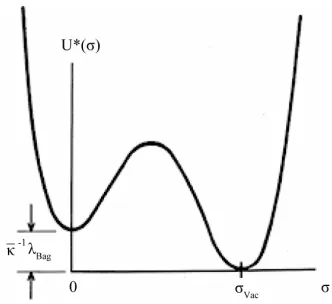
Next we come to another important point in this pic- ture. In modern cosmology, the notion of phase transi- tions plays a fundamental role. These involve SSB and contribute to the VED V. The consequence is that the effective vacuum potential U
responsible for SSB has two phases [48] and takes on two vacuum states. In hadron physics, there is the bag constant which represents an internal negative pressure that subtends the hadron (Figure 1, later). It is not the sameas
0 B
p B
vac
for the background in (7).
These multiple values of the gravitational APdS vacua are not space-time-dependent. Rather they are tempera- ture-dependent. They occur because the vacuum exists at a finite temperature produced by curvature-induced quantum corrections in gauge theories with scalar fields [49]. Spacetime thus has a chemical potential and is temperature-dependent in these asymptotic metrics for temperature T. It is the presence of thermal matter (had- rons) that breaks the Lorentz invariance of these vacuum states [50].
[image:5.595.340.506.83.235.2]Hence, during a phase transition in the early FLRW universe, the formation of hadrons has locally broken the
Figure 1. The two vacuum states of the cosmological con- stant
Bag
λ λvac
in the scalar-tensor model. The scalar
σ-field has undergone a phase transition and breaks the symmetry of the temperature-dependent vacuum, creating two vacuum states , and . Inside the hadron at
Bag 0,λ λ
. Outside the hadron at σvac , the
gravitational ground-state energy density of the vacuum Evac is defined by the background metric ημν in (7) with
F L
λλ for the Friedmann-Lemaitre accelerating universe.
Both are a de Sitter space.
Lorentz invariance of the global vacuum in (10). A local Lorentz boost and Poincaré translation from the outside of the hadron, into its interior, do not result in the same vacuum. This will become evident in Section 3.2.
Therefore, the fundamental basis for (9) and (10) can- not explain the existence of hadrons in the universe today. For this reason, we turn here to the original standard sca- lar-tensor theory [40-42] for an answer. The historical motivation for the JFBD theory was to create a time- dependent, variable gravitation constant G G t
. That is not the purpose here. Rather, the self-interacting scalar field ϕ will be regulated by the SSB process and must allow both G and λ to have two different states or values, one inside and one outside the hadron, that are tempera- ture-dependent. EG in (9) cannot accomplish this.
U 3.2. Symmetry Breaking Potentials
There are many examples of symmetry breaking poten- tials U
. These include the well-known quartic Higgs potential for the Higgs complex doublet
†
2U
†
2,2 0
0
(11)
where and
. (11) has minimum potential T
min 0, 2
2
energy for with . Viewed
as a quantum field, has the vacuum expectation value min
. Following SSB, one finds T
min 0, x 2
the Higgs particle η. In order to determine the mass of η
one expands (11) about the minimum min and obtains
2 2o
U U 3 1 4,
4
(12)
where 1 4 2 2
o
U is negative definite (wrong sign for solving the CCP), and η acquires the mass
2 2
m . Another example is the more general self- interacting quartic case
1 2 2o
U U m 3 4,
2 4!
c
(13)
investigated by [51,52] to examine the ground states of nonminimally coupled, fundamental quantized scalar fields ϕ in curved spacetime. Uo is arbitrary. (13) is based upon the earlier work of T.D. Lee et al. [39,53-57] and Wilets [58] for modelling the quantum behavior of had- rons in bag theory
2 3 4,
3! 4!
b c
2 2
o
d a
U U T (14)
where
U B
represents the self-interacting scalar
σ-field as a nontopological soliton (NTS).11
o is the bag constant and is positive. The work of Friedberg, Lee, and Wilets (FLW) is reviewed in [58-61]. See also [62].
In all cases (12)-(14), Uo represents a cosmological term,12 and all are unrelated except that they represent the VED of the associated scalar field. The terms in U
have a mass-dimension of four as required for renor- malizability. In the case of (11) and (12), it is the addition of the Higgs scalar η that makes the standard electroweak theory a renormalizable gauge theory. Also, the elec- troweak bosons obtain a mass as a result of their interac- tion with the Higgs field η if it is present in the vacuum.
Note finally that (11)-(14) all have the same basic quartic form. The focus here will be on the hadron bag (14) in FLW theory. As pointed out by Creutz [63,64] the bag is an extended, composite object subject to nonlocal dynamics and not subject to perturbation theory. Follow- ing symmetry breaking, the soliton bag potential is de- picted in Figure 1. The ground-state vacuum
at
c
va vac is the APdS background defined by in (7) as argued in Section 2 and is given by (1). The second vacuum state at 0 is internal to the hadron and is given by the bag constant B 1
Bag
is determinable by experimental hadron spectroscopy that models all hadrons, and is defined below.
On the other hand, quark and gluon confinement is generally attributed to the nonperturbative structure of the QCD vacuum. This is the basis for the MIT bag model [65,66] which first introduced B and visualized hadrons as bubbles of perturbative (PT) vacuum im- mersed in the nonperturbative (NP) QCD vacuum. In that case, a truly NP VED in Yang-Mills theory has been de- rived [67,68]. The difference between PT and NP vacua is by definition B, provided of course that someday back- reaction of the APdS spacetime is properly accounted for in QFT and QCD [69].
In what follows, we will show how to resolve CCP-1 in hadron physics using (14). This will be done in the fashion of a modified JFBD scalar σ nonminimally cou-pled to the tensor field g in (9).
3.3. Merging Hadrons with Gravity
As discussed regarding (14), λ in (9) is actually a potential term
that contributes to U
. In that manner it couples to the SSB self-interacting quartic fieldσ added to give QCD a scalar field [39] in the FLW bag model. However, here σ will be treated as a gravitational field in order to address CCP-1.
Matter will be limited to hadron bags and will be moved to become a part of the bag potential in (14) as U B 1
Bag
o
. This transposes λ to the right- hand side13 of (9) and gives the scalar-tensor field equ- ations
B
. o in (14) is not a bare parameter determinable by a calculation, any more than Uo in (12) derives a Higgs mass. B is a fundamental parameter of FLW bag theory,
U
1 ,
2
R g R T
, M
T T T
(15)
(16)
Bag B, (17)
where now T
contributes to the σ-field tensor
. The matter tensor is TM T in (9), and their
sum
T in (16) is conserved by the Bianchi identities.
We will derive T below using scalar-tensor methods. Note that (17) resolves the mass dimensionality of λ and B in that both sides of the equation have mass dimension two.
This amounts to moving λ about within the total La- grangian £ T U
S S S S
for the action involved,
Gravity Matter G M, . Recalling that the Lagrangian for the FLW bag model £FLW is that for QCD
£ £
£*q C supplemented by the nonlinear σ-field
plus a quark-σ mixing term £q
*
£ £ £ £ £ ,
,
(18) FLW q q C
11The asterisk in (14) is used to indicate that d0. T*σ is a chiral SB 0
d
term that represents the cloud of pions surrounding the bag. restores the symmetry.
12U
o in (13) and (14) is an absolute number that is not experimentally measurable. This will become apparent in the definition of B that follows.
13Geometry in EG is determined by g
μν—not which side of the equation
the £*
term here will become the σ-field interaction
term with scalar-tensor gravity G, *
£ £ in the total Lagrangian that includes a nonminimally coupled Ein- stein-Hilbert term as
£q £q £ ,C
JFBD £
Total JFBD
£ £ £ (19)
where
£G, , * 1£
2 U
£
[59
(20)
and JFBD will be introduced shortly as (27).
The σ-field may be interpreted as a gluon condensate arising from nonlinear interactions of the color fields £C
]. Regardless of its origin and composition, this scalar is the basis for the model under discussion.
For quarks ψ, scalar σ, and colored gluons C, these terms in (18) and (19) are
£q i D m , (21) £q f, (22)
14 2
1
£ c ,
C F F gs Ac (23) where counterterms are not shown. m is the quark flavor mass matrix, f the σ-quark coupling constant, gs the strong coupling, Fμν the non-Abelian gauge field tensor,
Dμ the gauge-covariant derivative, and
the gravi- tation-covariant derivative (also in Fμν) with the spin
connection derivable upon solution of (15) above, de- fining the geodesics.
is the phenomenological dielectric function introduced by Lee et al. [53-55], where
0 1 and
vac
0 in order to guarantee color confinement. The SU3 Gell-Mann matrices and structure factors are λc and fabc respectively.Variation of (18) which neglects gravity in (19), using (20)-(23), gives the FLW equations of motion for σ and
ψ,
' ,
U f
–m f– 0,
(24)
i D (25)if one neglects the gluonic contribution (23). □ is the curved-space Laplace-Beltrami operator, and
d d
U U is
2 3.
4 2 3!
d b c
U T a
0
d
(26)
A variant adopts to simplify (26) when pion physics is not involved.
In the same fashion that
1
is a function of the
σ-field, κ is likewise as . For purposes here, the original JFBD ansatz is adopted although there are others. This ansatz directly relates to (17). Taking into account (20), the nonminimally coupled scalar-
tensor Lagrangian is
JFBD
matter £
1
8π£ .
2 g R U
(27)
The task now is to complete the scalar-tensor picture. The energy-momentum tensor in (16) is comprised of two terms. The first is the usual matter contribution TM
which includes all matter fields in the universe except gravitation,
2 M M
M g L g L
T
g
g g
.
* £
(28)
It is thereby independent of the gravitational σ-field.14 The second term in (16) T g is new and must include the effects of G,
£ in (20). Con- solidating all of the σ terms and introducing a superscript “R” for renormalizable, we have in short-hand derivative notation
; ; ; ;
1 .
2
RT g g U
0 M
T
T
(29) With (28) and (29), variation of (27) will now give the final equations of motion.
A principal assumption follows Brans and Dicke (BD). In order not to sacrifice the success of the principle of equivalence in Einstein’s theory [11], only gμν and not σ
enters the equations of motion for matter consisting of particles and photons. The interchange of energy be- tween matter and gravitation thus must follow geodesics as assumed by Einstein [70]. Therefore, the energy- momentum tensor for matter is assumed to be conserved in the standard fashion, .15
;
The derivation of is a textbook problem [70] except that the latter was a classical treatment following BD—both of which neglected λ, any potential U
U
, and the renormalization restrictions on
;
; ; ; ; ;
.
T
A B C
D E g U
in (14). The most general symmetric tensor of the form (29) which can be built up from terms each of which involves two derivatives of one or two scalar σ-fields, and σ itself, is
; ; ; ; ; ;.
RT U
(30)
We want to find the coefficients A, B, C, D, and E. Taking the covariant divergence of (29) gives
matter
£
M
L
(31)
14In (28), .
and that of (30) results in
; ; ; ; ; 2 T A B A D A B D CE U U
; ; ; ; ; ;. C E 1 (32)Recalling the ansatz , next multiply (15) by σ
and take its divergence,
;
1 1
2 ; 2g R
; ;
8π M 8π .
R g R R
T T (33)
The first term on the l.h.s. of (33) is zero by the Bianchi identities; the first on the r.h.s is zero by the principle of equivalence. The net result is
; 8πT ; . 1
2
R g R
R
(34)
Using an identity [70] involving the Riemann tensor
;
; .0
f
, the first term in (34) is
; ; ; ; ; ; ;
R (35) Take the trace of (15) and (16) for R. Next modify (24) to include the gravitational coupling with σ (still assum- ing ) to produce the trace for TM. Lastly obtain the remaining trace for T from (30). These three traces are
, M
RT T
' ,
U
; ; 4 . B C D (36) 1 1 2 MT (37)
4 4 T A E U
1 ; ; 4 4 . C D E U (38)It follows that the collective trace for R is
1 2 ' 4 R UA B
(39)
Placing (39) into the left-hand-side of (34) with some re-arrangement gives
; ; ; ; 1 1 ; ; ; ; ; ; 1 1 ; 1 21 2 4
1 2 2
0 1 1
1 2 2 ' 4 .
R g R
A B
C D
U E U
E (40)In order that (34) be true, the bracketted coefficients in (32) and (40) must be equal term by term. Renor- malization problems created by are addressed in Ref. [71]. These include the insolvability of a quintic and the Galois-Abel theorem.16 Finally, one encounters the
result
11
1 2 3 2
A which prompts the de- finition 1 1 3, 2 1 (41)
in (37) is whereby
1
2 . 3 2
(42)
The desired energy-momentum tensor for the σ-field follows as
; ; ; ; 2 ; ; 1 2 1 1 . T gg g U
(43)
Inserting (43) into (15) and (16) gives the full field equations
; ; ; ; 2 ; ; 1 28π 1
2
1 1 ,
M
R g R
T g
g g U
0 f (44)
while (43) in (37) gives the scalar wave equation (for
) for the -field
8π ' ,
3 2 T U
(45)
where 1
1 3 2
and κ1 is the source of - coupling to the traditional trace TM in JFBD theory. There is now coupling to the trace in (45) compared to (24). If
T
3 2
, (44) is a conformally mapped set
of Einstein field equations.
E E 1
3.4. Characterizing Scalar-Tensor Gravity and Hadrons
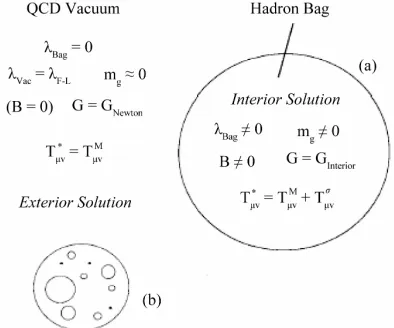
In order to visualize the results (44), (45), and (25), Fig- ure 2 illustrates this scalar-tensor approach to CCP-1.
Bag Boundary Conditions. Bag surface boundary con- ditions are discussed in Ref. [72], p. 103, where the fol- lowing can be adopted: Fn 0
0
for gauge fields; and
for quark fields. As a problem in bubble dynam- ics, one uses 1 4 J 1
Jn B
F F for a
quark current J and surface tension Σ. Alternatively the more recent Lunev-Pavlovsky bag with a singular Yang- Mills solution on the bag surface [73-76] can be utilized (also probably eliminating the need for
in (23), a point that is yet to be addressed).
From the dimensionality of U
U
in (14), we see that a has mass-dimension two or m2. Taking the deriva- tive as in (26) along with (45), the -field has
mass
.
m a
(46) Therefore it is a short-range field with only short- range interaction. (45) can be re-written
2
,
M
U 8π T f
3 2
m
U
e r m
(47)
[image:9.595.73.270.465.629.2]where is the remainder of (26) after moving the aσ term to the left-hand side. Hence a static solution must have a Yukawa cutoff where .
Figure 2. The existence of two vacuum states for
characterized by Equations (16), (44), (45), and (47). The exterior is traditional Einstein gravity where λλF L . (a)A single hadron bag is depicted with 1 Bag Bκ λ
T
; (b) The
general interior solution is depicted as a many-bag problem using a Swiss-cheese (modified Einstein-Straus) model with zero pressure on the bag surfaces. Applicable boundary conditions are in [72-76].
This is characterized in Figure 2 by indicating that the
energy-momentum tensor is confined to the hadron which is consistent with the original conjecture of FLW that the σ-field be related to confinement.
Bag Interior Conditions. By virtue of the bag condi- tion (17), several new features come into play. First, this relation is specific to the interior of the bag. Second, the BD ansatz 1G1
0
B
is now tied to the cosmologi- cal parameter λ too.17 This means that when the phase transition and SSB occur, there exist two de Sitter spaces in Figures 1 and 2. Both λ and G can differ between the
two vacuum states. When (no bags), vac
1
G
in Figure 1, restoring itself to the ground-state vacuum
of the APdS background (Section 2). Similarly,
G
is not guaranteed in theory to be the same in the hadron interior as Newton outside. This is a matter for experi- mental investigation (Section 4.2 below).
Summary. Semi-classically speaking, the scalar-tensor theory of gravity in the presence of the QCD Lagrangian representing FLW bag theory in (18) and (19) has no apparent problem associated with the existence of two vacuum states, one in the exterior and one in the interior of hadrons.
This model has been done entirely in de Sitter space, whereby the principle of compatible asymptotic Killing charges (Section 2) has not been broken. Thus, CCP-1 does not appear to apply to scalar-tensor gravity when nonminimally coupled to hadron physics. The model al- lows for two vacuum states, as bags indicate experimen- tally. One is the F-L ground state F L
and theother is the hadron interior Bag .
However, the issue of vacuum stability for this model is a crucial assumption because one can argue that it is unstable to radiative corrections. But radiative correc- tions have long been suggested as the origin of SSB to begin with [77]. These similarly are important for dy- namical SB (DSB) models as well [78,79]. Since SSB has been adopted for the basic quartic potential U
in (13) and (14), then there has been an implicit assump- tion that the scalar-tensor configuration presented here is stable to radiative corrections. Vacuum stability of this model is a subject for further study, in particular when QCD confinement is more thoroughly understood.
4. Cosmological Event Horizons, Finite
Temperature, and Experiment
The connection between λ and graviton mass (Appendix) has a bearing upon identifying the APdS spacetime as the ground state vacuum for the CCP with its associated Killing charges in the AD formalism, in order to rectify CCP-2 in Section 2. Because there exists the G-H event horizon in such cosmological spacetimes, any association
of λ with a graviton mass is very pertinent even if it is gauge dependent.
In the Appendix as (67), it is shown in the weak-field approximation that a graviton massmg 3 is asso- ciated with a small λ such as (1) for de Sitter spacetime. It is equivalent to the surface gravity C 3 found by G-H [25]. These in turn relate directly to the radius of the event horizon EH defined by the singularity in (2) and (3) at
r
1
EH C
Next, finite temperature effects must be discussed and this is done below in Section 4.1. Experimental aspects follow in Section 4.2 and are recapitulated in Table 1.
r
U
.
4.1. Finite Temperature Effects
A digression on the effect of finite temperature T upon
is pertinent because it is relevant to experiment. The subject is also pertinent to the basic concept of a temperature-dependent spacetime in gravitation theory, and equally so to the topic of cosmological event hori- zons.
The subject is treated in the usual fashion [80-82]. The classical, zero temperature potential U in (14) becomes V
U
VS
,T
VF
, ,T
. This
involves scalar VS and fermionic VF correction terms for chemical potential μ, by shifting σ as
T . The result is a temperature-dependent cosmological bag parameter [83,84]
,T
B
,T
B 0
Bag Bag which
decreases with increasing temperature T until the bag in
Figure 2 dissolves and symmetry is restored
in
Figure 1.
In such a case and in simplest form [85], the bag mo- del equations of state are
4 ,
SB
T k T B (48)
1 4 ,3k TSB B
p T (49)
2
π
30 SB
7 , 8
B F
k d d
0
T
(50)
[image:10.595.134.268.487.565.2]where energy density ε and pressure p now have a tem- perature dependence
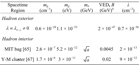
. The Stefan-BoltzmannTable 1. Summary of the masses, VED’s, and λ’s in space-time.
Spacetime
Region (cmmg−1) (eV)mg (GeV)mσ VED(GeV), B4 (cmλ−2)
Hadron exterior
0
F L
0.6 × 10⁻²⁸ 1.1 × 10⁻³³ 2 × 10−47 0.7 × 10−56
Hadron interior
MIT bag [65] 2.6 × 10⁻⁷ 5.2 × 10⁻¹² a 0.0045 2 × 10⁻¹³
Y-M cluster [67]1.7 × 10⁻⁶ 3 × 10⁻¹¹ a 0.02 9 × 10⁻¹²
(SB) constant kSB is a function of the degeneracy factors dB for bosons (gluons) and dF for fermions (quarks and antiquarks). The absence of the baryonic chemical poten- tial μ in (48) is a valid approximation for ongoing ex- periments involving nucleus-nucleus collisions. All are relevant to quark-hadron phase transitions and the quark- gluon plasma (QGP).
4.2. Experimental Aspects
As mentioned previously (Section 3), EG appears to be the correct theory of gravity above 1 mm. The subject here is below that scale in the Large Hadron Collider (LHC) realm of particle and nuclear physics. Granted, the treatment in this paper has neglected the standard model in order to present a tractable discussion of had- rons, gravity, and the CCPs.
Within the hadron bag. Here one has mg0 due to (17) and (67). Adopting a simplified view of the hadron interior and a bag constant value from one of the con- ventional bag models, the MIT bag [65,66] where
1 4 146 MeV
B B60 MeV fm 3 13 2
2 10 cm
B
Bag or , then
7 1 2.6 10 cm
m
follows from (17).18 Using (67) in the Appendix, a graviton mass g
12 5.2 10 eV 1 4 10 cm6
m
or is found within the bag. Although this appears to represent a Compton wavelength of
g or range of
1 2 10 cm6
m
1 2 g , it is
derived from Bag and is only applicable for the interior solution. This is depicted in Figure 2. It has no range
outside of the bag where Bag 0. 4
0.02 GeV
YM
B
12 2 8.7 10 cm
YM
A similar calculation for the Yang-Mills condensate
[67,68] gives
1.7 10 cm6 1
g
m
11
3 10 eV, and 1 2mand 13.5 10 cm 5 or N
G G G
Bag G g
Regarding G, adopting Bag ewton is the sensible assumption to make. However, Bag is a free parameter, independent of B. It has never been experimentally measured. For any B determined in Table 1, can
be anything except zero.19
.
The bag per se. The σ-field has a mass (46) in Table 1
subject to experimental measurement, perhaps at the LHC in scalar gluon jets related to ongoing boson searches to complete the Standard Model [86,87]. It is conceivable that evidence for both the Higgs boson and the scalar σ-field used here for the bag can be found.20 18In terms of units, the following conversions are helpful:
4 5 3
1 MeV 2.3201 10 gcm , then 1.8658 10 cmg 27 1 or
22 2 4
4.3288 10 cm MeV
. Thus 13 2
Bag B 2 10 cm
3 5 4
gcm 2.3201 10 MeV
B B
for
. This assumes G G Newton.
19This would move the Planck mass, M
Planck1 GBag .
20The recent suggestion of Friedberg and Lee [88] that the Higgs itself
[image:10.595.56.286.629.737.2]External to the hadron. By taking the well-known JFBD limit in (44) and (45), we in fact obtain Einstein gravity (for exceptions see Ref. [46]) due to the experimental limits [43-45]. The small graviton mass mg in (67), on the other hand, results in a finite-range gravity whose mass is g
2 3
m
10 28cm1 0.6
m 1 10 33eV
3
42 10 eV
1056cm2
or 1. .
This follows from the vacuum energy density
which is equivalent to , for the de Sitter background in (7) for the F-L
accelerating universe [7,8].
Obviously, Newton in the exterior.
Summary. The results for this model are as follows. In the exterior we have a graviton mass
and a range of
G G
28 1 10 cm
0.6
g
m
18 10 cm 27
1 1 2mg
which is approximately the Hubble
radius. That is, gravitation outside of the bag is finite- ranged reaching to the G-H cosmological event horizon
. Gravitation within the bag is short-ranged. C
Clearly the sign of λ must be positive (de Sitter space) in (67) in order that an imaginary mass not be possible. The latter represents an unstable condition with patho- logical problems such as tachyons and negative proba- bility. (67) is a physical argument against such a circum- stance.
EH
r
5. Assumptions and Postulates
At this point the fundamental postulates that have been made are summarized. These have been discussed and alluded to throughout but are now recapitulated.
1) Einstein gravity is the true theory of gravity at length scales above 1 mm.
2) The gravitational field g couples minimally and
universally to all of the fields of the Standard Model, as does Einstein gravity [11]. However, g also couples
nonminimally to the composite features of FLW and . The term represents hadron physics which
£ £
FLW£QCD 1
QCD FLW
includes QCD in the exact limit (see Ref. £
£ [59], p. 19). The JFBD ansatz
£
is assumed. 3) The nonlinear self-interacting scalar σ-field re- presented by Lagrangian is a gravitational field, because it couples universally to all hadronic matter. Since σ has a mass (46) it and T in (16) have a cutoff
and are confined to the hadron in Figure 2(a).
4) General covariance is necessary in order that the Bianchi identities determine conservation of energy- momentum from T in (15). However, in the hadron
exterior, T TM
0
f
. That means matter follows Einstein geodesics and obeys the principle of equivalence as expected there.
5) Stability must be assumed for δTμν in the Appendix.
Use of the harmonic gauge, in (53), suppresses
the vector gravitons and manifests a tiny graviton mass
g , but breaks general covariance. The con- sequence is not measurable within the observer’s cos- mological event horizon.
6) Temperature-dependent quantum vacuum fluctu- ations result in a broken vacuum symmetry, producing two distinct vacua containing two different vacuum energy densities F L and Bag. Lorentz and Poincaré invariance are broken by T in the interior of hadrons. Because
T , this broken symmetry is subject to restoration.7) The stability of the bag is assured by the vacuum energy density B which is a negative vacuum pressure. Similarly, the scalar-tensor representation of the hadron interior is stable against radiative corrections.
8) The principle of compatible asymptotic states (Kill- ing charges) is assumed. This means that the global ener- gies of flat ADM metrics are not compatible with those of APdS metrics. ADM energies cannot be consistently compared globally with AD energies in the definition of ground-state vacua for de Sitter space, lest infinities be introduced. Hence, derivations in flat Minkowski space are not relevant to the CCP if (1) is accepted as evidence for λ contributing to the acceleration of the universe in FLRW cosmology whose current phase is an APdS met-ric.
6. Conclusions
A tenable model for the origin of hadron bound states in bag theory has been shown to derive from the cos- mological constant λ in scalar-tensor gravity, noting that the familiar Higgs mechanism does not account for the mass of composite particles such as hadrons. The bag model of Friedberg, Lee, and Wilets (FLW) is used in- stead.
According to the development in Section 3, a scalar- tensor treatment of gμν nonminimally coupled to hadrons
using the nonlinear self-interacting scalar field σ results in a model of gravity that has two different ground-state vacua. Such a theory exists and resolves CCP-1 adopting the assumptions made here. Experiment and theory must eventually settle the differences between the MIT bag model and the Yang-Mills condensate solution for bag constant B in Section 3.2, but this does not alter these results. As a model, this point of view represents a ten- able strategy for reconsidering CCP-1 and CCP-2 from hadron physics to cosmology. Without directly relating the bag constant to the global energy in APdS spacetime, any of the other proposed “solutions” of the CCP(s) are incomplete.
breaks the principle of compatible asymptotic states, by comparing energies derived from spacetimes that have entirely different Killing charges and global energy pro- perties. A great deal of work on APdS structure and its relation to VEDs is therefore required before we will truly understand the CCP.
Finally, conventional massive gravity g PF has not been used in the strategy proposed here to address the CCP PF . This investigation involves only λ and its relationship to asymptotic infinity, with a graviton mass mg (65) and (67) that manifests itself by suppress- ing the vector gravitons fμ in (53). In this study, mg arises instead by introducing
m m
m 0
0
into the well-known Regge-Wheeler problem (see Appendix).
7. Acknowledgements
The author would like to acknowledge helpful commu- nications with B. Tekin, as well as O. V. Pavlovsky, S. J. Aldersley, and A. Waldron.
REFERENCES
[1] A. Einstein, Preussische Akademie der Wissenschaften, Sitzungsberichte, 1917, pp. 142-152.
[2] A. Einstein, Preussische Akademie der Wissenschaften, Sitzungsberichte, 1919, pp. 349-356.
[3] H. Weyl, “Raum-Zeit-Materie,” Springer, Berlin, 1922. [4] M. Bronstein, Physikalische Zeitschrift der Sowjetunion,
Vol. 3, 1933, pp. 73-82.
[5] G. Lemaitre, Proceedings of the National Academy of Sciences, Vol. 20, 1934, pp. 12-17.
doi:10.1073/pnas.20.1.12
[6] Ya. B. Zel’dovich, JETP Letters, Vol. 6, 1967, pp. 316-317
[7] A. G. Riess, A. V. Filippenko, P. Challis, et al., Astro- nomical Journal, Vol. 116, 1998, pp. 1009-1038. doi:10.1086/300499
[8] S. Perlmutter, G. Aldering, G. Goldhaber, et al., Astro- physical Journal, Vol. 517, 1999, pp. 565-586.
doi:10.1086/307221
[9] E. J. Copeland, M. Sami and S. Tsujikawa, International Journal of Modern Physics D, Vol. 15, 2006. pp. 1753- 1935. doi:10.1142/S021827180600942X
[10] S. Weinberg, Reviews of Modern Physics, Vol. 61, 1989, pp. 1-23. doi:10.1103/RevModPhys.61.1
[11] T. Damour, Journal of Physics G: Nuclear and Particle Physics, Vol. 37, 2010, p. 225.
[12] M. Maggiore, Physical Review D, Vol. 83, 2011, Article ID: 063514. doi:10.1103/PhysRevD.83.063514
[13] M. Maggiore, L. Hollenstein, M. Jaccard and E. Mitsou, Physics Letters B, Vol. 704, 2011, pp. 102-107.
doi:10.1016/j.physletb.2011.09.010
[14] L. F. Abbott and S. Deser, Nuclear Physics B, Vol. 195, 1982, pp. 76-96. doi:10.1016/0550-3213(82)90049-9
[15] S. Weinberg, “The Cosmological Constant Problems,” In: D. Cline, Ed., Sources and Detection of Dark Matter and Dark Energy in the Universe, Springer, New York, 2001, pp. 18-28. doi:10.1007/978-3-662-04587-9_2
[16] J. Garriga and A. Vilenkin, Physical Review D, Vol. 64, 2001, Article ID: 023517.
doi:10.1103/PhysRevD.64.023517
[17] F. Kottler, Annalen der Physik, Vol. 56, 1918, pp. 401- 462. doi:10.1002/andp.19183611402
[18] R. Arnowitt, S. Deser and C. Misner, “The Dynamics of General Relativity,” In: L. Witten, Ed., Gravitation: An Introduction to Current Research, John Wiley & Sons, New York, 1962, pp. 227-265.
[19] V. Faraoni and F. I. Cooperstock, Astrophysical Journal, Vol. 587, 2003, pp. 483-486. doi:10.1086/368258
[20] T. Shiromizu, Physical Review D, Vol. 49, 1994, pp. 5026-5029. doi:10.1103/PhysRevD.49.5026
[21] S. Deser and B. Tekin, Physical Review Letters, Vol. 89, 2002, Article ID: 101101.
doi:10.1103/PhysRevLett.89.101101
[22] S. Deser and B. Tekin, Physical Review D, Vol. 67, 2003, Article ID: 084009. doi:10.1103/PhysRevD.67.084009 [23] S. Deser and B. Tekin, Physical Review D, Vol. 75, 2007,
Article ID: 084032. doi:10.1103/PhysRevD.75.084032 [24] S. Deser, I. Kanik, and B. Tekin, Classical and Quantum
Gravity, Vol. 22, 2005, pp. 3383-3389. doi:10.1088/0264-9381/22/17/001
[25] G.W. Gibbons and S. Hawking, Physical Review D, Vol. 15, 1977, pp. 2738-2751. doi:10.1103/PhysRevD.15.2738 [26] H.W. Hamber, “Quantum Gravitation,” Springer, Berlin,
2009.
[27] I. L. Buchbinder, S. D. Odintsov and I. L. Shapiro, Ri-vista del Nuovo Cimento, Vol. 12, 1989, pp. 1-112. doi:10.1007/BF02740010
[28] K. S. Stelle, Physical Review D, Vol. 16, 1977, pp. 953- 969. doi:10.1103/PhysRevD.16.953
[29] K. S. Stelle, General Relativity and Gravitation, Vol. 9, 1978, pp. 353-371. doi:10.1007/BF00760427
[30] T. Padmanabhan, Classical and Quantum Gravity, Vol. 19, 2002, pp. 5387-5408.
doi:10.1088/0264-9381/19/21/306 [31] B. Tekin, Private Communication.
[32] K. A. Olive and J. A. Peacock, Journal of Physics G: Nu- clear and Particle Physics, Vol. 37, 2010, pp. 230-245. [33] E. Komatsu, K. Smith, M. Nolta, et al., Astrophysical
Journal Supplement, Vol. 180, 2009, pp. 330-376. doi:10.1088/0067-0049/180/2/330
[34] H.-J. Blome and T. L. Wilson, Advances in Space Re- search, Vol. 35, 2005, pp. 111-115.
doi:10.1016/j.asr.2003.09.056
[35] S. Weinberg, “Cosmology,” Oxford University Press, Oxford, 2008.
[36] C. M. Will, Living Reviews in Relativity, Vol. 9, 2006, pp. 3-100.