SLearn
: Shared learning human activity labels
across multiple datasets
Juan Ye
School of Computer Science, University of St Andrews, UK [email protected]
Abstract—The research of sensor-based human activity recog-nition has been attracting increasing attention over years as it is playing an important role in various human-beneficiary applications such as ambient assistive living, health monitoring, and behaviour changing. Nowadays, the advancement of sensing and communication technologies has led to the possibility of collecting a large amount of sensor data, however, to build a reliable computational model and accurately recognise human activities we still need the annotations on sensor data. Acquiring high-quality, detailed, continuous annotations is a challenging task. In this paper, we explore the solution space on sharing annotated activities across different datasets in order to enhance the recognition accuracies. We have designed and developed two approaches:sharing training dataandsharing classifierstowards addressing this challenge. We have validated the approach on three datasets and demonstrated their effectiveness in recognising activities only with annotations from as little as 0.1% of each dataset.
Index Terms—human activity recognition, smart home, active learning, transfer learning, uncertainty reasoning
I. INTRODUCTION
Sensor-based activity recognition has increasingly played a significant role in many applications, which enables to provide customised services to suit people’s current context; for example, better optimising energy by adjusting heaters based on users’ activity routine [4], understanding the impact of human behaviours to environmental phenomena such as the change of indoor air quality [12], or assessing physical and cognitive conditions of disadvantaged residents [23].
Human activity recognition has been a popular research topic in the last decade, and numerous machine learning, data mining, knowledge-driven techniques have been applied and achieved promising results at targeting various problems. However, challenges still remain, and a crucial challenge resides in the scarcity of annotated datasets. First of all, acquiring annotations from users can be a time- and effort-consuming task. The state-of-the-art activity recognition tech-nologies either use video to record activities of users, which will later be annotated by third parties, or rely on users’ self-report. The former approach has an undesirable privacy concern, while the latter can result in less accurate, incomplete annotations [26]; for example, users forget to record certain activities or use different terms to describe their activities.
Even though the recent attempts have helped to address the above challenges by facilitating self-annotation with the support of technologies [27] and enhancing the consistency of annotation labels via ontologies [19], acquiring annotations for
long-term activity recognition is still a challenging task. That is, we only collect ground truth over the training period (e.g., the first few weeks or months) so that the machine learning techniques can use the annotated training data to build models. After that, we assume that the models stay fixed and can be used continuously to recognise human activities in the long term (e.g, for a couple of years). However, this assumption does not consider the fact that human activity routine or activity pattern might change over time, users (or background users like visitors or even pets) might interact with sensors differently, or users might conduct new activities that have not been recorded at all during the training period; that is, they might behave differently from the training period to the actual system running period.
Therefore, acquiring annotations to enable long-term activ-ity recognition is one of the main challenges, and there have been different approaches proposed to address towards this problem. Unsupervised activity recognition is one way, where we either rely on common sense knowledge from the other sources (such as the Web or other textual sources [29] or domain knowledge [31]) to build activity profiles or build computationally expensive models to separate sensor data for each type of activities [22]. Another direction is active learning, where a classifier will build a computational model on a limited set of annotated data, and then iteratively annotate a large amount of un-annotated data. In each iteration, it will select uncertain data points that sit at the boundary of classes, and ask the human operators to annotate them so as to use them further train and refine the computational model. This approach can significantly reduce human annotation effort, however, it still requires all the activities of interest are covered in the initial annotated data. Recently transfer learning techniques are starting to attract attention and have also been applied to address this challenge. For example, a meta-feature space mapping technique has been developed to map sensors from one home environment to another so as to share the activity recognition model [5], but this approach can be subject to the density of sensors being deployed and the routines of activities from different users.
datasets, we are able to better recognise unlabelled examples than classic activity recognition approaches. The contribution of this paper is to propose algorithms for shared learning across activity recognition models from different users in different environments with different deployments of sensors. We evaluate the algorithms on three third-party datasets and demonstrate their effectiveness by comparing them against the state-of-the-art classification techniques.
The rest of the paper is organised as follows. Section II proposes the problem thatSLearnaims to address with formal definitions and an illustration example. Section III reviews the mainstream work on addressing the scarcity of labelled data and identifies the difference between them and SLearn. Section IV describes the SLearn approach and Section V introduces the evaluation methodology and experiment setup. Section VI performs an evaluation and discusses the strength and limitation, and Section VII concludes with some suggested future work.
II. PROBLEMSTATEMENT
In this section, we will introduce the research problem that the SLearntries to address, through a formal definition and a concrete illustrative example.
A. Formal Definition
Based on the syntax and terminology from transfer learn-ing [16], we first give preliminary definitions of problems that the SLearnapproach aims to address.
Definition 1. Let a datasetDS consist of a domainD and a task T, where
• a domain D is a two-tuple (χ,P(X)). χ is the feature
space of DandP(X)is the marginal distribution where
X = [x1, ..., xn]∈χ.
• a taskT is a two-tuple(Y, f())for a given domainD.Y
is the label space of D, which is a collection of possible labelsY ={y1, y2, ..., ym}.f()is an objective predictive function for D.
• Within this dataset, each pair (X, y) ∈ χ×Y ∪ {Θ}, whereΘrepresentsunknownorunlabelled. That is, some instances in the feature space have labels; i.e., (X, y)∈
χ×Y andf(X)∈Y, while the other instances do not; i.e., (X,Θ)∈χ× {Θ} andf(X) = Θ.
Definition 2. Let DSS be a collection of datasets
{DS1, DS2, ..., DSL}, where each dataset has different
do-mains (i.e., ∀1≤i, j ≤L,i6=j,χi 6=χj andPi6=Pj) and has different tasks (i.e.,Yi6=Yj andfi6=fj).SLearnaims to assign a label to each unlabelled instance in the dataset; that is, ∀X ∈ χi, there exists a label y ∈Y1∪Y2∪...∪YL. To make it work, there are two assumptions:
• Feature space remapping - the feature spaces between these datasets are comparable and can be remapped be-tween each other. That is, there exists a mapping function
θi,j :χi→χj that remaps each instance X inχi to an
instance X0 inχj.
• Label space remapping- the label spaces between these
datasets are comparable and can be remapped between each other. That is, there exists a mapping functionϑi,j:
Yi→Yj that remaps each labely inYi to a labely0 in
Yj.
B. An Illustrative Example
Here we will illustrate the above definitions through an example of theSLearnscenario, which is activity recognition in a smart home environment deployed with binary event-driven sensors. Assume we deploy sensors in two different home settings:House I andHouse II. Due to different spatial layout and users’ preference, we deploy a different number of sensors with different sensing technologies in these two environments. For example, one house is deployed with a dozen of infra-red passive motion sensors, indicating the user’s whereabout, while the other house is deployed with switch sensors to monitor the open/close states of cupboards, doors, or windows, and the pressure sensors to indicate whether a user sits on sofa or sleeps in bed.
When the sensors are deployed, we can start activating a SLearn Algorithm, without the need for explicit training period, as the training is continuously ongoing. Both users can start annotating their activities at their own pace. For example, if the user in House I has annotated a few examples of “preparing breakfast” and the user in House II has annotated a few examples of “taking bath”, then the SLearnAlgorithm aims to recognise these two activities in both House I and II. It will support long-term incremental activity recognition in that it can accommodate new activities annotated by different users over time.
III. RELATEDWORK
Activity recognition has been an active research topic in the last decade, and a large number of knowledge- and data-driven techniques have been proposed [30]. Among them, different approaches have been designed to address the scarcity chal-lenge of activity annotation, including unsupervised learning, activity learning, and transfer learning. In the following, we will compare and contrast these approaches with SLearn.
A. Unsupervised Learning
from the work in [18], they have applied the generic ontologies to automatically map the discovered sensor sequential patterns to activity labels through a semantic matching process [31]. Yordanova et al. have also applied domain knowledge in rule-based systems to generate probabilistic models for activity recognition [11], [33].
Taking a different route, researchers also have applied web mining and information retrieval techniques to extract the common-sense knowledge between activities and objects via mining online documents; that is, what objects are used to perform a daily activity and how significant each object is contributed to identifying this activity [15], [29], [32], [34]. During the reasoning process, the mined objects are mapped to sensor events and an appropriate activity will be recognised. SLearn is not a classic activity recognition problem where for each dataset we train a model with labelled instances and recognise unlabelled instances. In SLearn, the training data is assumed to be incomplete in that it might not cover all the activities of interest.SLearnis not a unsupervised learning technique as it still relies on labelled training data, but the labels can come from different datasets.
B. Active Learning
Active learning, so called “query learning”, is a subfield of machine learning, which is motivated by the scenario when there is a large amount of unlabelled data but a limited and insufficient amount of labelled data. As the labelling process is tedious, time-consuming and expensive in real-world applications, active learning methods are employed to alleviate the labelling effort by selecting the most informative instances to be annotated [20].
Alemdar et al. apply active learning strategies to select the most uncertain instances to be annotated; that is, the instances sit at the boundaries of different activity classes [1]. The annotated instances are then used to iteratively update a HMM to infer daily activities in a home setting. Their experimental results have demonstrated that active learning strategies have improved recognition accuracies, compared to random selection. Cheng et al. apply a density-weighted method that combines both uncertainty and density measure into an objective function to select the most representative instances for user annotation, which has been demonstrated to improve activity recognition accuracy with the minimal labelling effort [3]. Similarly, Hossain et al. combine the un-certainty measure and Silhouette coefficient to select the most informative instances as a way to discover new activities [8]. SLearn is not an active learning problem [20] in that it will not query a user or a human operator, but learns labels from the other datasets. However, we could use the uncertainty sampling strategies in active learning to determine when an algorithm should leverage training data or classifiers from other datasets.
C. Transfer Learning
Transfer learning is another approach to deal with the limitation of labelling data, where knowledge learned from
a source domain (with labelled data) can be transferred to a target domain (without labelled data) [16].
Zheng et al. [34] propose an algorithm for cross-domain activity recognition that transfers the labelled data from a source domain to a target domain so that the activity model in the source domain can help to complete the similar ac-tivity model in the target domain. The similarity is not only measured on the objects being involved in the activities, but also on their underlying physical actions. One example is that the activity ‘Washing-laundry’ is similar to “Hand-washing dishes” on the action of “Hand washing”. They use the web search and apply the information retrieval techniques to build the similarity function that produces different probabilistic weights of actions and objects on activities of interest. These weights will be further used to train a multi-class weighted support vector machine to support activity recognition.
Maekawa et al. [13] have proposed an unsupervised ap-proach to recognise physical activities from accelerometer data. They utilise information about users’ characteristics such as height and gender to compute the similarity between users, and find and adapt the models for the new users from the similar users.
van Kasteren et al. [24] propose a manual mapping between sensors in different households and learn the parameters of a target model using the EM algorithm to transit probabilities of HMM models from source to target. Similarly, Rashidi et al. [17] learn sensor mappings based on their locations and roles in activity models. The role is characterised in mutual information, measuring the mutual dependence between an activity and a sensor and suggests the relevance of using the sensor in predicting the corresponding activity. Feuz et al. [5] propose a data-driven approach to automatically map sensors based on their meta-features, which are mainly about when a sensor reports, and time intervals between events reported by this sensor and other sensors.
SLearn is most relevant to but not the same as transfer learning [16]. Our assumption is slightly different from the above works where they assume a complete model (that is, containing all the activities of interest) can be learnt on a source domain, while we assume each domain can only have a small fraction of data being annotated (that is, the activities having been annotated can be a subset of activities of interest in a domain) and we do not assume any domain necessarily as a source or target domain. However, transfer learning techniques such as feature remapping can be applied to SLearn. Especially, our approach is most similar to the above three, where we focus on sensor mappings to support sharing sensor data across multiple datasets. The difference is that we are using a knowledge-driven approach where sensors are modelled in location and object ontologies whose generality across different households and sensing technologies has been demonstrated in other works [31].
D. Co-training
performance of a learning algorithm by leveraging a large number of unlabelled examples [2]. The idea is that the de-scription of each example can be partitioned into two distinct views, and each view can be linked with edges in a bipartite graph. Then two classifiers can be trained separately on each view, and then results from each classifier are used to enlarge the training set of the other. The co-training algorithm and its variations have been recently applied in the multi-view human activity recognition in smart home environments [6]. That is, an activity can be viewed from different platforms of sensor streams, such as acceleration data, motion sensor, or video. The principle is to learn the same activities from each sensor platform and share and adapt labels from one sensor platform to another. For example, a home is equipped with ambient sensors to monitor motion, lighting, temperature, and door use. The resident now wants to train smart phone sensors to recognise the same activities on ambient sensors. Whenever the phone is located inside the home, both sensing platforms collect data while activities are performed, resulting in a multi-view learning opportunity where the ambient sensors represent one view and the phone sensors represent the other view. If the phone can be trained, it can also monitor activities outside of the home and can update the home’s model when the resident returns. The phone may converge upon a stronger model than the home either because it receives training data of its own or because it has a more expressive feature space.
The SLearn problem does not share the same assumption as the co-training approach in that the co-training approach works on multiple views from the same data while the SLearn approaches need to work on multiple datasets that share the sensing mission; that is, compatible sensor features and activities.
IV. PROPOSED APPROACH
We hypothesise that we can significantly improve activity recognition accuracies by leveraging a small set of training data contributed from each dataset. All these datasets might have a different number of sensors, in different sensing technologies, deployed in different environments, and from different users, as long as they have compatible feature space and activities of interest. The contributed training data might only contain a couple of examples, and possibly not cover the whole set of activities of interest. In the following, we will explore the solution space to address this question.
First of all, a classic approach of dealing with a small amount of training data is leveraging unlabelled data, which is similar to the active learning approach, mentioned in Sec-tion III-B. That is, for each dataset, we train a classifier on its labelled data and then use it to iteratively infer the labels on its unlabelled examples for T rounds or until the algorithm converges. For each iteration, we select the top k
most confident examples to enlarge the labelled data pool and iteratively update the classifier. However, given our assumption that the labelled data might be too little and have not covered the whole set of activities of interest, this basic approach can only assign the labels that have been observed in the training
data. We will need to leverage labels from the other datasets. To do so we will look into two directions: sharing training data and sharing classifiers.
A. Sharing training data
To share training data, we will need to map data from the feature space of one dataset to the feature space of the other dataset. An intuitive approach is feature-space remap-ping in transfer learning; that is, convert an instance XI =
[xI,1, xI,2, ..., xI,nI]from a dataset I to a representation in
an-other dataset II:θI,II(XI) =XII = [xII,1, xII,2, ..., xII,nII]. There are different feature remapping strategies introduced in [16]. Feuz et al. [5] have proposed a meta-feature based mapping function for event-driven sensors in smart home environments. They have defined a range of meta-features about each sensor; for example, the average sensor event frequency over 1-hour time periods, over 3/8/24-hour periods, the mean and standard deviation of the time between this sensor event and the next sensor event, and the probability of the next event is from the same sensor. These meta-features are used as a heuristic to guide the mapping process. This is a data-driven approach for feature-space remapping, but its performance might be affected by the activity routine of various users and the deployment and types of sensing technologies in each environment. For example, one user might often have breakfast at 6am while the other might have at 9am, or one user prefers having shower before breakfast while the other prefers the other way around so that the sensors might be mis-matched on the time scale. In addition, the density of the sensor deployment and the frequencies and sensitivity of sensors reporting events might affect the mapping on the intervals between events. For example, one environment can be more densely deployed with sensors so that the time distances between events reported by different sensors can be significantly shorter than the other set up with much fewer sensors.
To reduce the impact of such differences in each dataset, we will adopt a more general approach - semantics-based feature mapping. We will use the common knowledge [31], which has demonstrated generality across different smart home datasets. The principle of semantics-based feature mapping is to compute similarity between a pair of sensors based on where they are deployed and which object they have attached to. Both location and object concepts are organised in an ontological hierarchy, from which a conceptual similarity measure [28] is applied to calculate the distance between two concepts. Here we re-apply the conceptual ontologies to feature re-mapping.
Definition 3. Given an instanceXI = [xI,1, xI,2, ..., xI,nI], a semantics-based feature mapping function is defined as
θ(XI) = XII, denoted as [xII,1, xII,2, ..., xII,nII], where
∀1≤j≤nII,xII,j=Pi∈Sjxi∗sim(sI,i, sII,j)/|Sj|,Sj is
a collection of sensors in the feature space I that are similar to the sensorj in II.
Sj={sl|1≤l≤nI, sim(sI,l, sII,j)> ε},
sim(sI,l, sII,j) =wL×simL(sI,l, sII,j) +wO×simO(sI,l, sII,j),
where ε is the threshold to choose similar sensors, simL
and simO are the similarity measure on location and object concepts that the lth sensor in I and j sensor in II, and wL
andwO are the weights on the location and object similarity.
Based on the above definition 3, a valuexII,jin a converted instance XII ∈χII is the weighted average of the probabili-ties of all the similar sensors in the source feature spaceχI to thejth sensor inχII and the weight is their sensor similarity. That is, we try to estimate the probability of the jth sensor reporting events by looking at the probabilities of all of its similar sensors in the source dataset.
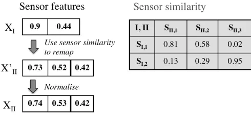
Figure 1 illustrates an example of the above process. As-sume that there are two datasets I andII, each having 2 and 3 sensors respectively, and their similarity scores have been calculated based on the similarity of their attached objects and deployed locations. Given a current sensor feature XI
in the dataset I, we need to simulate a sensor feature XII
[image:5.612.51.296.383.497.2]in the other dataset. First, for each sensor in II, we need to identify similar sensors in I. Assume that the similarity threshold is 0.5, according to the formula in Definition 3, we identify the similar sensor sets Sj(j = 1,2,3) for each sensor in the dataset II as {sI,1},{sI,1}, and {sI,2}. Then the probability on each sensor is the averaged contribution from their similar sensors. The location and object ontologies as well as the sensor similarity calculation can refer to the work [31].
Fig. 1: An example of sensor feature space remapping
With feature remapping, for each dataset, we will not only train a classifier on its own train data but also on the data converted from the training data in the other datasets. This gives rise to Algorithm 1.
B. Sharing classifiers
To share classifiers, we design a uncertainty-driven algo-rithm; that is, when the classifier from the current dataset cannot confidently infer an activity label to a given example, then we acquire labels from the classifiers from the other datasets. This is inspired by active learning; that is, identify uncertain examples and query human operators for annotation. The difference here is that we don’t query human operators, but classifiers in the other datasets. The process is described inSC Algorithm.
To make SC Algorithm work, we will need to solve two questions: (1) how to evaluate whether an example is uncertain
Algorithm 1 SD: Share training Data
Require: a collection of datasets {D1, D2, ..., Dn}, where each
dataset Di is composed of a set of labelled examples Li and
a set of un-labelled examplesUi
1: initialise a classifierCifor each dataset
2: fort= 1 doT
3: Lci →Li∪ {Lj|L0 0j=remap(Lj, i), j6=i, j∈[1, n]}
4: use labelled examples in each datasetLci to train its classifier
Ciand estimate an uncertainty measureµi
5: randomly create a set of {U0
1, U20, ..., Un}0 from un-labelled
examples
6: useCi to label Ui0 and select k most confident and certain
examplesKi
7: Li→Li∪Ki
8: Ui→Ui−Ki
9: end for
Algorithm 2 SC: Share Classifiers
Require: a collection of datasets {D1, D2, ..., Dn}, where each
dataset Di is composed of a set of labelled examples Li and
a set of un-labelled examplesUi
1: initialise a classifierCifor each dataset
2: fort= 1 doT
3: use labelled examples in each datasetLito train its classifier
Ciand estimate an uncertainty measureµi
4: randomly create a set of {U0
1, U 0 2, ..., U
0
n}from un-labelled
examples
5: foreach unlabelled exampleu∈Ui0 do
6: prob←Ci classifiesuand returns its class probabilities
7: ifµi evaluatesprobto be uncertainthen
8: use{C1, ..., Cn}to classifyuand integrate the results
9: end if 10: end for
11: selectk most confident and certain examplesKifromUi0
12: Li→Li∪Ki
13: Ui→Ui−Ki
14: end for
to label, and (2) how to integrate results from multiple classi-fiers. To address the first question, we will employ the most common uncertainty sampling strategies from active learning, which are least confidence, margin sampling, and entropy, as described in Equation 1, 2, and 3 respectively [20].
1) least confidence:
φ(x)LC = argmax
x
1−Pθ(ˆy|x) (1)
where yˆ = argmax x
Pθ(y|x) denotes the class label
assigned with highest posterior probability. A larger value ofφ(x)LC denotes a higher uncertainty.
2) margin sampling:
φ(x)M = argmin
x
Pθ(ˆy1|x)−Pθ(ˆy2|x) (2)
which computes the difference between two highest pos-terior probabilities. A smaller value of φ(x)M (smaller margin) denotes a higher uncertainty, suggesting it is hard to differentiate two most probable class labels. 3) entropy:
φ(x)E= argmax
x
−X
i
where entropy of each instance measures uncertainty of the corresponding set of posterior probabilities for all class labels. A larger value of φ(x)E denotes a higher uncertainty.
With the uncertainty sampling strategies, we can determine which example is not certain to be labelled from its current classifier. Then we will perform a feature space remapping that converts it to an example in the other datasets to allow the other classifiers to label. Once the other classifiers complete the inference, we will need to integrate their results to make a final decision. There are existing approaches to combine classifiers; for example, ensemble methods like boosting, bagging, and stacking are classic ways to do. However, we are constrained by the size of training data, so we propose a uncertainty-driven approach. It selects themost certainactivity label from each classifier in the other datasets and the process is described in Algorithm 3. To do so, we will reuse the above uncertainty sampling strategies on the inference results and calculate their uncertainty score with the above formulas.
Algorithm 3 CC: Combine Classifiers
Require: an unlabelled exampleu
Require: Classifiers {C1, C2, ..., Cn} and uncertainty measure
{µ1, µ2, ..., µn}for each dataseti∈[1, n]
1: initialiseres to store the inference results
2: foreach classifierCido
3: prob←Ciclassifiesuand returns its class probabilities
4: ifµievaluatesprobto be certainthen
5: add[cls, conf, us]tores, whereclsis the inferred class
label,conf is the probability oncls, andus is the uncertainty
score.
6: end if 7: end for
8: ifresis not emptythen
9: return[cls, conf]with the lowest uncertainty score fromres
10: end if
V. EVALUATION METHODOLOGY
We hypothesise that SD and SC Algorithms can significantly improve activity recognition accuracies when the available training data is very little. To validate this hypothesis, we design the following methodologies.
Datasets We use three real-world smart home datasets that capture typical activities and more importantly they represent common types of smart home datasets in terms of the number of sensors, different spatial layouts, and the degree of inherent noise. We believe that experimenting on these datasets gives us a comprehensive view of the effectiveness of the proposed technique. The three datasets were collected by the University of Amsterdam (named House A, B, and C respectively in the following) from three real-world, single-resident houses which were instrumented with wireless sensor networks [9]. These three datasets recorded the same set of 7 activities, including leaving the house, preparing breakfast or dinner, and sleeping. These three houses are deployed with only binary sensors, whose reading indicates whether or not a
sensor fires. More specifically, the House A dataset consists of 14 state-change sensors attached to attached to household objects like doors, cupboards, and toilet flushes, while the other two datasets contain more than 20 sensors, including reed switches to measure whether doors and cupboards are open or closed; pressure mats to measure sitting on a couch or lying in bed; mercury contacts to detect the movement of objects (e.g., drawers); passive infrared to detect motion in a specific area; float sensors to measure the flush of toilet.
AccuracyWe consider two metrics for accuracy: the overall accuracy – the ratio of the learnt labels being the same as the true labels, and the class accuracy – the averaged ratio of the learnt labels being the same as the true labels in each class.
Ao=|pred label==true label|
N
Ac=
P
c={1,...,C}(|pred labelc==true labelc|) P
c={1,...,C}(Nc)
,
whereC is the number of classes and Nc is the number of
test examples in each classc.
ProcessWe evaluate the algorithms across different ratios of training data, from 0.1% to 80%. 0.1% is the extreme training data percentage for the chosen datasets; that is, the training data for each dataset can only contain 1 or 2 examples. To validate our hypothesis, we want to observe the effectiveness of the proposedSDandSCAlgorithms when training data is very little and find to what percentage of training data both algorithms need to be able to produce satisfactory accuracies. For each given ratio r of training data, we randomly generater×Ni number of instances in the ith dataset to be
annotated, run an algorithm on all the datasets, and calculate the averaged class accuracies. The algorithms include the proposed SD and SC Algorithms as well as the baseline approach; that is, train a classifier with training data of each dataset and test on its test data, without any sharing data or classifiers. We run 100 iterations for each ratio, test all these algorithms on each iteration, and average their accuracies.
Uncertainty sampling strategiesWe have experimented with the three uncertainty sampling strategies in Section IV-B. For each strategy, we need to estimate the threshold to determine whether inferred class probabilities are uncertain or not. A general way to do is to split the training data into training and validation sets so that we can experiment with different thresh-old values and test on the validation set, and we choose the best threshold that leads to the highest accuracies. However, we are dealing with very small training data, we cannot afford the validation set. What we have done is that after training a classifier, we calculate the uncertainty scores of each training example and use the mean score as the threshold. For the extreme case with only one training data, we set the default threshold score on the most uncertain situation; that is, evenly distributed class probabilities. Also we allow the uncertainty threshold to be updated during the iterative training phase, so the default threshold only serves at the cold start stage.
In terms of combining classifiers, we have evaluated CC Algorithm and compared with the classic ensemble methods such as majority voting (MV) and highest confidence (HC) and Dempster-Shafer Theory (DST) to integrate imperfect evidences from distinct sources [14]. The MV, HC, and DST have similar results, all worse than SC Algorithm as they are more likely to be affected by the weaker classifiers. CC Algorithm with the information entropy uncertainty sampling strategy produces the highest performance.
Top k example selection In both SD and SC Algorithms we will need to choose top k examples for the next training iteration. We have experimented with different numbers 2, 5, and 10. Both top 2 and 5 produce better accuracies as they only focus on best examples while filtering less confident ones. For the sake of performance, we will choose top 5, which leads to faster convergence.
VI. RESULTS ANDDISCUSSION
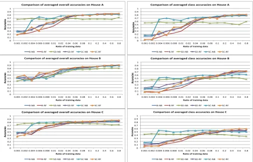
This section will discuss the evaluation results and validate our hypothesis. Figure 2 presents the comparison of overall and class accuracies between Baseline, SD, and SC Algorithms on each dataset.
SD and SC Algorithms improve both overall and class accuracies when the ratio of training data is small; i.e., from 0.1% to 10%, and perform comparably with the base-line approaches afterwards. To quantify the improvement, we perform significance tests on the performance of SD, and SC Algorithms over the Baseline Algorithm with their corresponding base classifiers respectively. For each ratio of training data, we run Welch’s t test on the accuracies of 100 iterations and calculate the p-values, which are presented in Figure 3. With a null hypothesis H0 ofSD, andSCproviding no improvement overBin recognising activities, and an alter-native hypothesis H1 ofSD, andSC displaying improvement, we select a standard significance level of 90% for the test, meaning that if the p-value in the test result is smaller than 0.1, we reject the null hypothesis and accept that there is a
statistically significant improvement. The result in Figure 3a shows that when the training ratio is less than 1%, SD has significantly improved the overall and class accuracies (not on RF) with the p-values all close to 0. The main reason is that accumulating training data from multiple sources does provide better coverage. Again in the extreme situation, if training data from each dataset contains one example from different classes, then collecting them together will cover three classes. When the training data is small,SDAlgorithm with NB works much better than RF; that is, the averaged class accuracies of 55% with NB and of 17% with RF on House A when the ratio of training data is 0.1% in Figure 2. The reason is that RF often needs more training data to compose a number of decision tree classifiers and less sensitive to small change in training data, while NB is built on a much simpler model and can adapt well to small change in training data.
As presented in Figure 2, the improvement over the class accuracies are more observable. We can see that even when the ratio of training data is only 0.1%, the overall accuracies on the baseline approaches can be as high as 50%, especially on House B and C. After looking into the inference results, we find that on these two datasets, if the training data only contains the high frequency activities, such as the “leave house” and “sleep” activities that dominate the House B and C datasets, then both the classifiers NB and RF will only predict these two activities, leading to the final overall accuracies to be the actual class distribution. Also because these activities have higher frequency, during the iterations, they are more likely to be chosen in the training data, which leading to a high overall accuracy. As suggested by the authors of the datasets [25], the class accuracies are more indicative on the actual performance of the classification techniques. In the following, we will focus on our discussion on the class accuracies.
SD Algorithm is less sensitive to the amount of training data; for example on House A, the averaged class accuracy is 55% at the lowest ratio 0.1%, and 59% at the highest ratio 80% in Figure 2. When the ratio of training data increases, SD Algorithm performs worse than B and SC Algorithms. It suggests that when training data is sufficient, sharing data across different datasets does not help, but adds noise to the classifiers in each dataset. Partly it is because each user tends to have their own way or routine of performing certain activities; for example, interacting with different objects. Sharing data can enhance activity coverage, but not necessarily improve identifying activities for individual users.
improve-0 0.1 0.2 0.3 0.4 0.5 0.6 0.7 0.8 0.9 1
0.001 0.002 0.004 0.006 0.008 0.01 0.02 0.04 0.06 0.08 0.1 0.2 0.4 0.6 0.8
Ac
cu
ra
cie
s
Ratio of training data
Comparison of averaged overall accuracies on House A
B-NB B-RF SD-NB SD-RF SC-NB SC-RF
0 0.1 0.2 0.3 0.4 0.5 0.6 0.7 0.8 0.9 1
0.001 0.002 0.004 0.006 0.008 0.01 0.02 0.04 0.06 0.08 0.1 0.2 0.4 0.6 0.8
Ac
cu
ra
cie
s
Ratio of training data
Comparison of averaged class accuracies on House A
B-NB B-RF SD-NB SD-RF SC-NB SC-RF
0 0.1 0.2 0.3 0.4 0.5 0.6 0.7 0.8 0.9 1
0.001 0.002 0.004 0.006 0.008 0.01 0.02 0.04 0.06 0.08 0.1 0.2 0.4 0.6 0.8
Ac
cu
ra
cie
s
Ratio of training data
Comparison of averaged overall accuracies on House B
B-NB B-RF SD-NB SD-RF SC-NB SC-RF
0 0.1 0.2 0.3 0.4 0.5 0.6 0.7 0.8 0.9 1
0.001 0.002 0.004 0.006 0.008 0.01 0.02 0.04 0.06 0.08 0.1 0.2 0.4 0.6 0.8
Ac
cu
ra
cie
s
Ratio of training data
Comparison of averaged class accuracies on House B
B-NB B-RF SD-NB SD-RF SC-NB SC-RF
0 0.1 0.2 0.3 0.4 0.5 0.6 0.7 0.8 0.9 1
0.001 0.002 0.004 0.006 0.008 0.01 0.02 0.04 0.06 0.08 0.1 0.2 0.4 0.6 0.8
Ac
cu
ra
cie
s
Ratio of training data
Comparison of averaged overall accuracies on House C
B-NB B-RF SD-NB SD-RF SC-NB SC-RF
0 0.1 0.2 0.3 0.4 0.5 0.6 0.7 0.8 0.9 1
0.001 0.002 0.004 0.006 0.008 0.01 0.02 0.04 0.06 0.08 0.1 0.2 0.4 0.6 0.8
Ac
cu
ra
cie
s
Ratio of training data
Comparison of averaged class accuracies on House C
[image:8.612.53.560.48.373.2]B-NB B-RF SD-NB SD-RF SC-NB SC-RF
Fig. 2: Comparison of averaged overall and class accuracies between Baseline,SD, andSCAlgorithms, showing SDand SCAlgorithms
can improve recognition accuracies when training data are small.
0 0.1 0.2 0.3 0.4 0.5 0.6 0.7 0.8 0.9 1
0.001 0.002 0.004 0.006 0.008 0.01 0.02 0.04 0.06 0.08 0.1 0.2 0.4 0.6 0.8
p-value
Ratio of training data
Significance test of accuracies between baseline and SD algorithms on House A
NB - Overall Accuracies NB - Class Accuracies RF - Overall Accuracies RF - Class Accuracies
(a) B vs. SD
0 0.1 0.2 0.3 0.4 0.5 0.6 0.7 0.8 0.9 1
0.001 0.002 0.004 0.006 0.008 0.01 0.02 0.04 0.06 0.08 0.1 0.2 0.4 0.6 0.8
p-value
Ratio of training data
Significance test of accuracies between baseline and SC algorithms on House A
NB - Overall Accuracies NB - Class Accuracies RF - Overall Accuracies RF - Class Accuracies
[image:8.612.61.561.403.517.2](b) B vs. SC
Fig. 3: Significance test on the performance between Baseline, SD, and SC Algorithms, showing SD and SC Algorithms can improve
recognition accuracies when training data are small andSD works better thanSCAlgorithm.
ment than SD. Secondly, the small training data significantly undermines the estimation of the uncertainty threshold. This becomes a more severe problem on RF than NB, as both classifiers produce very different class probabilities in the face of uncertainty. For example, under the extreme situation that there is only one example in the training data, saying it belongs to the 2nd class, for any test example, RF will derive the class probabilities [0,1,0,0,0,0,0]; that is, no matter which class the test example might belong, it will assign the highest probability 1.0 to the observed class in the training. On the contrary, NB will derive evenly distributed class probabilities
[0.14,0.14,0.14,0.14,0.14,0.14,0.14]. As introduced before,
we hardcode the uncertainty threshold as the most uncertain class probabilities, which can detect an uncertain example for
labelling on NB but not on RF. This raises a question on what heuristics we should use to better estimate uncertainty measures, which will be one of our future work.
0 0.1 0.2 0.3 0.4 0.5 0.6 0.7 0.8
0.9 1
0.001 0.002 0.004 0.006 0.008 0.01 0.02 0.04 0.06 0.08 0.1 0.2 0.4 0.6 0.8
Ac
cu
ra
cie
s
Ratio of training data
Comparison of class accuracies on different ways of sharing classifiers on House A
SC-NB SC2-NB SC-RF SC2-RF
[image:8.612.316.562.605.709.2]Due to this problem, we are also wondering what if we always share classifiers; that is, for each unlabelled example, we query all the classifiers and integrate their results. The results are presented in Figure 4, where SC2 refers to the always-sharing algorithm. With always sharing classifiers, SC2 Algorithm improves on RF, but not on NB. The results confirm our analysis that the poorer performance on RF is mainly to do with the uncertainty evaluation.
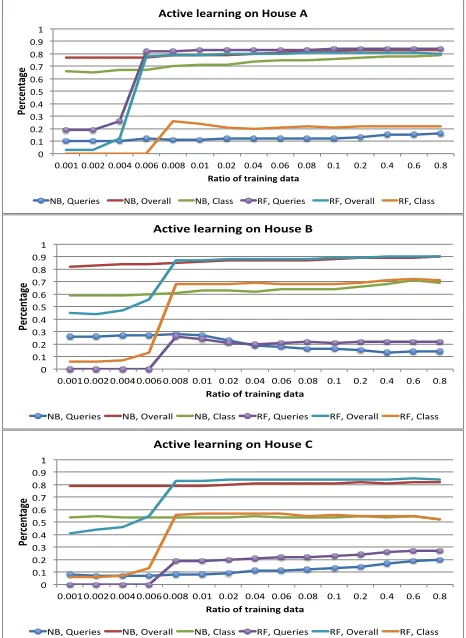
Comparison with active learningHere we will also compare the performance ofSDandSCAlgorithms with active learning in Section III-B, one of the most applied semi-supervise learning techniques in activity recognition. The performance of active learning with the information entropy uncertainty sampling strategy is presented in Figure 5, including the times of queries to acquire labels on uncertain examples from human operators and the overall and class accuracies. Compared to the results in Figure 2, active learning achieves better accuracies, however, it requires query 10% or 20% of test data to human operators, which makes the actual amount of training data is actually much higher than the specified. Also active learning assumes the alwaysavailability of true labels for each user’s own sensor data. On the one hand, this allows annotating sensor data for individual users and thus improves their own activity recognition model. On the other hand, it has better coverage of the activity space than our proposed methods in that the labels that we share in SD and SC are constrained by their availability in the other datasets’ training data. For example, if all the datasets only contain “having a meal” and “sleeping” activities altogether, then our techniques will not be able to detect any activities other than these two, but the active learning technique will still be able to learn the others such as “taking shower” or “having drink” because of the always availability assumption.
VII. CONCLUSION ANDFUTUREWORK
This paper aims to address the problem on the scarcity of activity annotations by leveraging annotations across different datasets that can have different sensing technologies, differ-ent sensor deploymdiffer-ent, and differdiffer-ent users, as long as they share the same mission with compatible sensor features and activities of interest. The goal of this paper is to explore the solution space to address the problem of SLearnand validate whether the proposed approach can improve activity recogni-tion accuracies given a small ratio of training data and if so, to what degree. To do so, we have proposed two approaches: SD Algorithm – accumulating a larger training data pool by semantically remapping training data from each other, and SCAlgorithm – acquiring and integrating activity labels from classifiers on the other datasets. We have presented the general skeletons of these two types of algorithms, and plugged in specific classifiers, feature space remapping techniques, and ensemble methods.
The evaluation results have consistently demonstrated a significant improvement on activity recognition accuracies when training data is small; for example, each dataset only
0 0.1 0.2 0.3 0.4 0.5 0.6 0.7 0.8 0.9 1
0.001 0.002 0.004 0.006 0.008 0.01 0.02 0.04 0.06 0.08 0.1 0.2 0.4 0.6 0.8
Percen
ta
ge
Ratio of training data Active learning on House A
NB, Queries NB, Overall NB, Class RF, Queries RF, Overall RF, Class
0 0.1 0.2 0.3 0.4 0.5 0.6 0.7 0.8 0.9 1
0.001 0.002 0.004 0.006 0.008 0.01 0.02 0.04 0.06 0.08 0.1 0.2 0.4 0.6 0.8
Percen
ta
ge
Ratio of training data Active learning on House B
NB, Queries NB, Overall NB, Class RF, Queries RF, Overall RF, Class
0 0.1 0.2 0.3 0.4 0.5 0.6 0.7 0.8 0.9 1
0.001 0.002 0.004 0.006 0.008 0.01 0.02 0.04 0.06 0.08 0.1 0.2 0.4 0.6 0.8
Percen
ta
ge
Ratio of training data
Active learning on House C
[image:9.612.321.554.37.356.2]NB, Queries NB, Overall NB, Class RF, Queries RF, Overall RF, Class
Fig. 5: Performance of active learning: times of queries vs. recogni-tion accuracies
contributes 2 or 3 annotated examples (i.e., the ratio of training data is 0.4%), the averaged class accuracies can reach around 66%, 52%, and 55% on House A, B, and C respectively. These algorithms can save a smart home system a large amount of time and effort on collecting ground truth. They can also potentially support lifelong learning of activity models as long as users from different smart home environments can contribute a few examples of their new activities, which can be either shared by SD Algorithm with the system in the other smart home environments or integrated bySCAlgorithm when similar sensor data are reported in the other home environments.
REFERENCES
[1] H. Alemdar, T. L. van Kasteren, and C. Ersoy. Using active learning to allow activity recognition on a large scale. InInternational Joint Conference on Ambient Intelligence, pages 105–114. Springer, 2011. [2] A. Blum and T. Mitchell. Combining labeled and unlabeled data with
co-training. In Proceedings of the Eleventh Annual Conference on Computational Learning Theory, COLT’ 98, pages 92–100, New York, NY, USA, 1998. ACM.
[3] H.-T. Cheng, F.-T. Sun, M. Griss, P. Davis, J. Li, and D. You. Nu-activ: Recognizing unseen new activities using semantic attribute-based learning. InProceeding of the 11th annual international conference on Mobile systems, applications, and services, pages 361–374. ACM, 2013. [4] P. Cottone, S. Gaglio, G. L. Re, and M. Ortolani. User activity recognition for energy saving in smart homes. Pervasive and Mobile Computing, 16(Part A):156 – 170, 2015.
[5] K. D. Feuz and D. J. Cook. Transfer learning across feature-rich heterogeneous feature spaces via feature-space remapping (fsr). ACM Trans. Intell. Syst. Technol., 6(1):3:1–3:27, Mar. 2015.
[6] K. D. Feuz and D. J. Cook. Collegial activity learning between heterogeneous sensors.Knowledge and Information Systems, 53(2):337– 364, Nov 2017.
[7] T. Gu, Z. Wu, X. Tao, H. K. Pung, and J. Lu. epsicar: An emerging patterns based approach to sequential, interleaved and concurrent activity recognition. In 2009 IEEE International Conference on Pervasive Computing and Communications, pages 1–9, March 2009.
[8] H. S. Hossain, N. Roy, and M. A. A. H. Khan. Active learning enabled activity recognition. In2016 IEEE International Conference on Pervasive Computing and Communications (PerCom), pages 1–9. IEEE, 2016.
[9] T. L. M. Kasteren, G. Englebienne, and B. J. A. Kr¨ose. Human activity recognition from wireless sensor network data: Benchmark and software. In L. Chen, C. D. Nugent, J. Biswas, J. Hoey, and I. Khalil, editors, Activity Recognition in Pervasive Intelligent Environments, volume 4 of Atlantis Ambient and Pervasive Intelligence, pages 165–186. Atlantis Press, 2011.
[10] H.-C. Kim and Z. Ghahramani. Bayesian classifier combination. In Pro-ceedings of the 15th International Conference on Artificial Intelligence and Statistics, 2012.
[11] F. Kruger, M. Nyolt, K. Yordanova, A. Hein, and T. Kirste. Com-putational state space models for activity and intention recognition. a feasibility study.PLOS ONE, 9:1–24, 11 2014.
[12] B. Lin, Y. Huangfu, N. Lima, B. Jobson, M. Kirk, P. OKeeffe, S. N. Pressley, V. Walden, B. Lamb, and D. J. Cook. Analyzing the relation-ship between human behavior and indoor air quality.Journal of Sensor and Actuator Networks, 6(3), 2017.
[13] T. Maekawa and S. Watanabe. Unsupervised activity recognition with user’s physical characteristics data. In2011 15th Annual International Symposium on Wearable Computers, pages 89–96, June 2011. [14] S. Mckeever, J. Ye, L. Coyle, C. Bleakley, and S. Dobson. Activity
recognition using temporal evidence theory. J. Ambient Intell. Smart Environ., 2(3):253–269, Aug. 2010.
[15] P. Palmes, H. K. Pung, T. Gu, W. Xue, and S. Chen. Object relevance weight pattern mining for activity recognition and segmentation. Perva-sive and Mobile Computing, 6(1):43–57, Feb. 2010.
[16] S. J. Pan and Q. Yang. A survey on transfer learning.IEEE Transactions on Knowledge and Data Engineering, 22(10):1345–1359, Oct 2010. [17] P. Rashidi and D. J. Cook. D.j.: Multi home transfer learning for resident
activity discovery and recognition. InIn: KDD Knowledge Discovery from Sensor Data, pages 56–63, 2010.
[18] P. Rashidi, D. J. Cook, L. B. Holder, and M. Schmitter-Edgecombe. Discovering activities to recognize and track in a smart environment. IEEE Transaction on Knowledge and Data Engineering, 23(4):527–539, Apr. 2011.
[19] M. Schr¨oder, K. Yordanova, S. Bader, and T. Kirste. Tool support for the online annotation of sensor data. In Proceedings of the 3rd International Workshop on Sensor-based Activity Recognition and Interaction, iWOAR ’16, pages 9:1–9:7, New York, NY, USA, 2016. ACM.
[20] B. Settles. Active learning literature survey. Computer Sciences Technical Report 1648, University of Wisconsin–Madison, 2009. [21] E. Simpson, S. Roberts, I. Psorakis, and A. Smith. Dynamic Bayesian
Combination of Multiple Imperfect Classifiers, pages 1–35. Springer Berlin Heidelberg, Berlin, Heidelberg, 2013.
[22] A. Vahdatpour, N. Amini, and M. Sarrafzadeh. Toward unsupervised activity discovery using multi-dimensional motif detection in time series. In Proceedings of the 21st International Jont Conference on Artifical Intelligence, IJCAI’09, pages 1261–1266, San Francisco, CA, USA, 2009. Morgan Kaufmann Publishers Inc.
[23] E. J. Van Etten, A. Weakley, M. Schmitter-Edgecombe, and D. Cook. Subjective cognitive complaints and objective memory performance influence prompt preference for instrumental activities of daily living. Gerontechnology : international journal on the fundamental aspects of technology to serve the ageing society, 14(3):169–176, 2016. [24] T. L. M. van Kasteren, G. Englebienne, and B. J. A. Kr¨ose.
Trans-ferring knowledge of activity recognition across sensor networks. In P. Flor´een, A. Kr¨uger, and M. Spasojevic, editors, Proceedings of the 8th International Conference on Pervasive Computing, pages 283–300, Berlin, Heidelberg, 2010. Springer Berlin Heidelberg.
[25] T. L. M. van Kasteren, G. Englebienne, and B. J. A. Kr¨ose. Human Activity Recognition from Wireless Sensor Network Data: Benchmark and Software, pages 165–186. Atlantis Press, Paris, 2011.
[26] J. A. Ward, P. Lukowicz, and H. W. Gellersen. Performance metrics for activity recognition. ACM Trans. Intell. Syst. Technol., 2(1):6:1–6:23, Jan. 2011.
[27] P. Woznowski, E. Tonkin, P. Laskowski, N. Twomey, K. Yordanova, and A. Burrows. Talk, text or tag? InPerCom 2017 Workshops, pages 123–128, March 2017.
[28] Z. Wu and M. Palmer. Verbs semantics and lexical selection. In Pro-ceedings of the 32nd annual meeting on Association for Computational Linguistics (ACL ’94), pages 133–138, Stroudsburg, PA, USA, 1994. Association for Computational Linguistics.
[29] D. Wyatt, M. Philipose, and T. Choudhury. Unsupervised activity recognition using automatically mined common sense. InProceedings of the 20th National Conference on Artificial Intelligence - Volume 1, AAAI’05, pages 21–27. AAAI Press, 2005.
[30] J. Ye, S. Dobson, and S. McKeever. Situation identification techniques in pervasive computing: a review. Pervasive and mobile computing, 8:36–66, Feb. 2012.
[31] J. Ye, G. Stevenson, and S. Dobson. Usmart: An unsupervised semantic mining activity recognition technique.ACM Trans. Interact. Intell. Syst., 4(4):16:1–16:27, Nov. 2014.
[32] K. Yordanova. From textual instructions to sensor-based recognition of user behaviour. InCompanion Publication of the 21st International Conference on Intelligent User Interfaces, IUI ’16 Companion, pages 67–73, New York, NY, USA, 2016. ACM.
[33] K. Yordanova and T. Kirste. A process for systematic development of symbolic models for activity recognition. ACM Trans. Interact. Intell. Syst., 5(4):20:1–20:35, Dec. 2015.