Uncertainty shocks in a model of effective demand : comment

Model of Effective Demand: Comment

∗

Oliver de Groot

Alexander W. Richter

Nathaniel A. Throckmorton

A

Basu and Bundick (2017) show an intertemporal preference volatility shock has meaning-ful effects on real activity in a New Keynesian model with Epstein and Zin (1991) preferences. We show when the distributional weights on current and future utility in the Epstein-Zin time-aggregator do not sum to1, there is an asymptote in the responses to such a shock with unit intertemporal elasticity of substitution. In the Basu-Bundick model, the intertemporal elastic-ity of substitution is set near unelastic-ity and the preference shock only hits current utilelastic-ity, so the sum of the weights differs from1. We show when we restrict the weights to sum to1, the asymptote disappears and preference volatility shocks no longer have large effects. We examine several different calibrations and preferences as potential resolutions with varying degrees of success.

Keywords: Stochastic Volatility, Epstein-Zin Preferences, Uncertainty, Economic Activity JEL Classifications: D81, E32

∗_{de Groot, School of Economics and Finance, University of St Andrews, St Andrews, Scotland and}

1 I

Basu and Bundick (2017)—denoted BB—build a New Keynesian model with time-varying de-mand uncertainty to replicate the effects of uncertainty shocks from an estimated VAR. An impor-tant contribution of their paper is to show that demand uncertainty shocks can generate meaningful declines in output and positive comovement between consumption and investment.1 _Demand un-certainty is modeled as a stochastic volatility shock to a representative household’s intertemporal preferences within an Epstein and Zin (1991) recursive preference specification. Preference shocks in expected utility settings have become a popular way to model changes in demand. However, the literature offers almost no guidance on how to introduce those shocks with recursive preferences.

We show when a preference shock is introduced in Epstein-Zin preferences and the distribu-tional weights on current and future utility in the time-aggregator do not sum to 1, there is an asymptote in the response to the shock with unit intertemporal elasticity of substitution (IES). In the BB model, the shock only hits current utility, so the sum of the weights differs from1. As a result, demand uncertainty shocks can generate arbitrarily large declines in real activity as the IES approaches unity from below and arbitrarily large increases as the IES tends to unity from above.2 The standard deviation of the preference shock is set to 0.003 in the BB model to match the volatility of real activity in the data. Given that value, the asymptote only has a meaningful effect on the responses to preference volatility shocks if the IES is near unity. BB set the IES to0.95, which is close enough to significantly magnify the size of the responses. For example, a one standard deviation preference volatility shock causes output to decline by0.13%on impact, whereas an IES set to 0.8 would have caused output to decline by only 0.025%. In contrast, an IES set to 1.05

would have caused output to increase by 0.14% on impact.3 _{Despite the importance of the IES,} there is no consensus about its value, which ranges from near0to2in the literature.4 _{In that range,} the BB model is able to generate responses to preference volatility shocks with any size and sign.

We show the asymptote disappears with preferences where the weights on current and future utility are restricted to sum to1. Unlike the BB preferences, the CES time-aggregator over cur-rent and future utility in our alternative specification is Cobb-Douglas as the IES approaches unity consistent with Epstein and Zin (1991) and Hansen and Sargent (2008, section 14.3). As a result, the model’s predictions become robust to small changes in the IES. There are also two important economic implications of our alternative preferences. One, demand uncertainty shocks have very small real effects. Two, output and investment increase and they no longer positively comove with consumption. Higher capital adjustment costs, risk-aversion, or price-adjustment costs can attenu-ate the increases in output and investment. However, only extreme parameter values restore the

co-1_{BB complement a large literature on uncertainty shocks (Bachmann et al. (2013), Bloom (2009), Born and Pfeifer} (2014), Fern´andez-Villaverde et al. (2015, 2011), Justiniano and Primiceri (2008), and Mumtaz and Zanetti (2013)).

2_{Albuquerque et al. (2016) add preference shocks to Epstein-Zin preferences the same way as BB, creating a similar}

asymptote. IES values slightly above (below) unity result in an arbitrarily large positive (negative) equity premium. 3_{Justiniano and Primiceri (2008) estimate a similar model with several sources of stochastic volatility and find}

time-varying volatility from a preference shock does not have a meaningful effect on output volatility. Similarly, Richter and Throckmorton (2017) estimate a nonlinear model where uncertainty arises from stochastic volatility as well as the state of the economy. They find a risk premium uncertainty shock reduces real GDP by less than0.01%.

movement and the magnitude of the responses remain much smaller than with the BB preferences. We examine two potential ways to restore the BB results with a lower IES. One, we retain the BB preferences and increase the steady state standard deviation of the preference shock. In that case, lower IES values generate responses to demand uncertainty shocks with a similar size as BB, but that occurs because the larger standard deviation effectively widens the influence of the asymptote. Two, we modify the preferences to exploit the observational equivalence between preference and disaster risk shocks following Gourio (2012). With an IES very close to0, disaster risk-type preference shocks can restore the BB results, but our finding is very sensitive to the value of the IES and also requires much higher risk aversion and price-adjustment cost parameter values. The paper proceeds as follows. Section 2 describes the BB preferences and our alternative specification.Section 3analytically solves an endowment economy to provide intuition for how the preference specification affects equilibrium dynamics.Section 4compares the two specifications in the full New Keynesian model.Section 5discusses two potential resolutions.Section 6concludes.

2 R

U

P

S

We begin by showing how the preference shock specification in an Epstein and Zin (1991) utility function affects the asymptotic properties of the value function and the household’s optimality conditions. In BB, the household chooses sequences of consumption,ct, and labor,nt, to maximize

U_tBB = [at(1−β)u(ct, nt)(1

−σ)/θ

+β(Et[(UtBB+1)1

−σ

])1/θ]θ/(1−σ)

, 16=ψ >0, (1)

whereθ ≡ (1−σ)/(1−1/ψ), σ ≥ 0determines the coefficient of relative risk aversion,ψ ≥ 0

is the intertemporal elasticity of substitution,β ∈ (0,1)is the subjective discount factor, andEtis

the mathematical expectation operator conditional on information in periodt.5 The current period consumption-leisure basket is defined asu(ct, nt) =cηt(1−nt)1−η, whereηdetermines the Frisch

elasticity of labor supply. The coefficient on current utility,at, is a preference shock that follows

at = (1−ρa) +ρaat−1+σ

a t−1ε

a

t, 0≤ρa <1, εat ∼N(0,1),

σ_ta = (1−ρσa)σa+ρ

σaσa

t−₁+σ

σa

εσ_ta, 0≤ρσa <1, εσ a

t ∼N(0,1),

The preference shock standard deviation, σa

t, follows its own process to introduce time-varying

demand uncertainty into the model, where σa

t and εat are uncorrelated. In contrast, the original

Epstein and Zin (1991) preference specification does not have an intertemporal preference shock. Given (1), the stochastic discount factor (SDF) that prices any1-period asset is given by

mBB_t,t+1 =β

at+1

at

u(ct+1, nt+1)

u(ct, nt)

1−σ

θ

ct

ct+1

(VBB t+1)1

−σ

Et[(VtBB+1)1

−_σ

]

1−1

θ ,

whereVBB

t is the value function that solves the household’s constrained optimization problem.

The utility function in (1) is constructed from two components. One, a time aggregator that characterizes preferences over the current consumption-leisure basket and the certainty equivalent of future utility. Two, a risk aggregator that controls preferences for risk over future utility. We focus on the specification of the time aggregator. Whenat = 1for all t, the time aggregator is a

CES function with distributional weights1−βandβ, respectively. The CES function then has the typical property that the time aggregator is Cobb-Douglas when the IES equals1so (1) becomes

U_tBB =u(ct, nt)1

−β

(Et[(UtBB+1)1

−σ

])β/(1−σ)

, ψ= 1, at= 1for allt. (2)

Given the transformationVBB

t ≡log(UtBB), (2) is more familiarly written as

VtBB = (1−β) logu(ct, nt) +βlog(Et[exp((1−σ)VtBB+1)])/(1−σ). (3)

However, ifat 6= 1, the distributional weights,at(1−β)andβ, no longer sum to 1. As a result,

preferences are undefined whenψ = 1and have the following properties as the IES approaches1:6

lim

ψ→1−

U_tBB = 0 (∞)forat>1 (<1) and lim ψ→1+

U_tBB =∞(0)forat >1 (<1).

To remove the asymptote, we propose an alternative to (1), where the distributional weights on current and future utility sum to1for allat ∈(0,1/β). The alternative specification is given by7

U_tALT =

(

[(1−atβ)u(ct, nt)(1

−σ)/θ

+atβ(Et[(UtALT+1 )1

−σ

])1/θ_]θ/(1−σ)

for16=ψ >0 u(ct, nt)1

−atβ

(Et[(UtALT+1 )1

−σ

])atβ/(1−σ)

forψ = 1 (4)

and the SDF becomes

mALT_t,t+1 =atβ

1−at+1β

1−atβ

u(ct+1, nt+1)

u(ct, nt)

1₋σ θ

ct

ct+1

(VALT t+1 )1

−σ

Et[(VtALT+1 )1

−σ

]

1−1

θ .

In sharp contrast with the BB preferences, the alternative specification becomes Cobb-Douglas and is therefore well-defined when the IES equals1.8 _{The analogous formulation to (3) is given by}

V_tALT = (1−atβ) logu(ct, nt) +atβlog(Et[exp((1−σ)VtALT+1 )])/(1−σ). (5)

The “risk-sensitive” preferences studied by Hansen and Sargent and others in the context of model uncertainty are not generalizable to preference shocks in the spirit of BB, but they are with (5).

To calibrate the new preference shock, we use expected utility preferences (σ = 1/ψ) because then the value function does not appear in the SDF. The log-linear SDF in each model is given by

ˆ

mBB_t,t+1 = ˆat+1−ˆat+ (1−σ)(ˆut+1−uˆt) + ˆct−ˆct+1,

ˆ

mALT_t,t+1 =−(βaˆt+1−ˆat)/(1−β) + (1−σ)(ˆut+1−uˆt) + ˆct−ˆct+1,

so we scale the standard deviations of the level and volatility shock by1−β and flip the sign of the shocks. The online appendix shows the two specifications generate nearly identical responses to first moment preference shocks but large differences in the responses to second moment shocks.

6_{The distributional weights must sum to1whenatis random but not when it is fixed since there is a transformation} of the value function that eliminates the asymptote and leaves the SDF unchanged. See the online appendix for details. 7_{Kollmann (2016) has a time-varying discount factor in a recursive preference setting similar to our formulation.} 8_{Rudebusch and Swanson (2012) rewrite Epstein and Zin’s preference specification asU}RS

t = (1−β)v(ct, nt) + β(Et[(URS

t+1)1−α])1/(1−α). That formulation is particularly useful when using utility kernels,vt, that are additively separable inctandnt. RS and BB preferences are equivalent whenv(ct, nt) ≡ u(ct, nt)(1−σ)/θ_{,α ≡ 1−θ, and}

3 I

This section presents a simple endowment economy model with an analytical solution to isolate the effect of the preference specification on equilibrium outcomes across IES values. The two specifi-cations, BB and ALT, are given in (1) and (4), respectively, exceptη = 1so labor is inelastically supplied. We assume the household receives a unit endowment in all periods except period 1 and can only save in period 0 at an exogenous rate,r. The preference shockat = 1in all periods except

period 1, where it equalsaH _{= 1 + ∆with probabilitypanda}L _{= 1−∆with probability1−p.}

SinceVt= 1fort≥2, the household’s problem reduces to choosingcBB0 orcALT0 to maximize

VBB

0 = [(1−β)(cBB0 )(1

−_σ)/θ

+β(E0[(a1(1−β)(cBB1 )(1

−_σ)/θ

+β)θ_])1/θ_]θ/(1−_σ)

or

V₀ALT = [(1−β)(cALT₀ )(1−σ)/θ

+β(E0[((1−a1β)(cALT1 )(1

−σ)/θ

+a1β)θ])1/θ]θ/(1

−σ)

,

subject tocj₁ =r(1−cj₀),j ∈ {BB, ALT}. The respective equilibrium conditions are given by

1 =βrE0

"

a1

cBB

0

cBB

1

1/ψ

(VBB

1 )1

−_σ

E0[(V1BB)1

−σ

]

1−1

θ#

(6)

or

1 =βrE0

"

1−a1β

1−β

cALT

0

cALT

1

1/ψ

(VALT

1 )1

−σ

E0[(V1ALT)1−σ]

1−1

θ#

, (7)

whereVBB

1 = [a1(1−β)c(1

−σ)/θ

1 +β]θ/(1

−σ)

andVALT

1 = [(1−a1β)c(1

−σ)/θ

1 +a1β]θ/(1−σ). With one equilibrium condition and one unknown,cj₀, we use a nonlinear solver to find the exact solution. Without any uncertainty (a1 = 1for allt), period-0consumption is given by¯cj0 =r/(r+ (βr)ψ).

0 0.2 0.4 0.6 0.8 1 1.2 1.4 1.6 1.8 2

IES (ψ) -0.02

-0.01 0 0.01 0.02

C

o

n

su

m

p

ti

o

n

(%

)

BB Preferences

Alternative Preferences

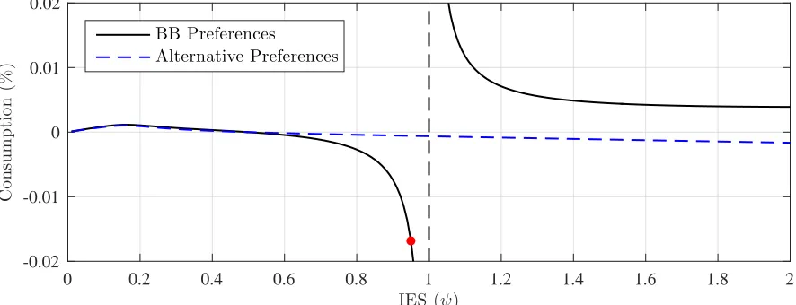
Figure 1: Period-0consumption as a percent deviation from the no-uncertainty level of period-0consumption. The circle marker shows the effect of uncertainty when the IES is0.95(BB value). The vertical line shows the asymptote.

0.5, and the amount of uncertainty,∆, to0.02. We scaleaH_andaL_{by1−βfor our alternative}

pref-erences so the results are almost identical for a deterministic change ina1. With expected utility, consumption is certainty equivalent, so both lines cross the horizontal axis whenψ = 1/σ= 0.5.

With the BB preferences, the relationship between period-0consumption and the IES features an asymptote at unit IES. As the IES tends to1, the effect of uncertainty is magnified. When the IES is slightly below unity, uncertainty leads to arbitrarily large declines in consumption, whereas an IES slightly above unity generates the opposite result. With our alternative preferences there is no asymptote, so the results are robust to small changes in the IES. The predictions from the two spec-ifications are very similar whenψ < 1/σ (i.e., ψ < 0.5withσ = 2). In that case, the household prefers a late resolution of uncertainty. In the more typical region of the parameter space where the household prefers an early resolution of uncertainty, the predictions of the two specifications quickly diverge. Unlike the BB preferences, the alternative specification induces precautionary behavior in response to uncertainty and the effect on consumption is small, regardless of the IES.

To better understand what is driving the results infigure 1, we rewrite (6) and (7) as

1 = ˜βj_r(cj

0/c

j

1)1/ψ,

where β˜j _{is an augmented discount factor due to the combination of recursive preferences and}

preference uncertainty. DefiningW₁j ≡(V₁j)1/ψ−σ

, the augmented discount factor is given by

˜

βj ≡β× E0[W

j

1]

(E0[(W1j)θ/(θ−1)])(θ−1)/θ

| {z }

Risk Aversion Term

× 1 + cov0(˜a

j

1, W

j

1)

E0[W1j]

!

| {z }

Covariance Term

, (8)

where˜aBB

1 =a1 and˜a1ALT = (1−a1β)/(1−β). Although the last two terms depend on the value of period-1consumption, the online appendix shows the effect is small. For simplicity, we evaluate

˜ βj _atcj

1 = βr/(1 +β), which is the no-uncertainty level of period-1consumption when ψ = 1. With expected utility preferences (i.e.,σ = 1/ψ), the value function drops out of the equilibrium condition in (6) or (7). As a result,β˜j _{=βand the asymptote disappears. In this case, whether one}

uses the BB or our alternative preference specification is inconsequential for equilibrium outcomes.

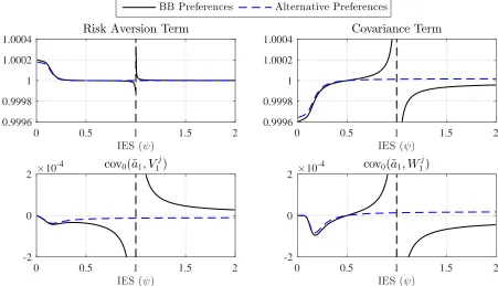
Figure 2 plots the decomposition of the augmented discount factor shown in (8). Comparing the vertical scales in the top left and top right panels reveals the variation in the augmented discount factor is mainly due to the covariance term and not the risk-aversion term. Looking at the bottom left panel, we can trace the source of the asymptote to the covariance between a1 andV1BB. In contrast, with our alternative preferences the covariance is always negative and modestly sized.

We conclude this section by showing two comparative statics that are useful for understanding the results from the BB model in the next section. Figure 3 shows the effect of increasing risk-aversion (left panel) and the amount of uncertainty (right panel). A higher risk risk-aversion parameter boosts the response of consumption for all values of the IES, so the domain in which the asymptote affects the responses is larger. Therefore, it is possible to lower the IES away from 1 and still generate the same consumption response by increasing risk aversion. SinceWBB

1 ≡(V1BB)1/ψ

−σ

, a higher σ increases the covariance term in the augmented discount factor. Higher uncertainty expands the influence of the asymptote in a similar way by increasing the covariance term. With our alternative preferences that eliminate the asymptote, higher uncertainty and risk aversion also increase the consumption response, but the magnitude is small compared to the BB preferences.9

0 0.5 1 1.5 2 IES (ψ)

0.9996 0.9998 1 1.0002

1.0004 Risk Aversion Term

0 0.5 1 1.5 2

IES (ψ) 0.9996

0.9998 1 1.0002

1.0004 Covariance Term

0 0.5 1 1.5 2

IES (ψ) -2

0 2 ×10

-4 cov0(˜_{a1, V1}j)

0 0.5 1 1.5 2

IES (ψ) -2

0 2 ×10

-4 cov0(˜_{a1, W1}j)

BB Preferences Alternative Preferences

Figure 2: Key terms in the decomposition of the augmented discount factor given in (8), wherej∈ {BB, ALT}.

0 0.5 1 1.5 2

IES (ψ)

-0.12 -0.08 -0.04 0 0.04 0.08 0.12

C

on

su

m

p

ti

on

(%

)

Risk Aversion (σ)

BB (σ= 2)

BB (σ= 5)

ALT (σ= 2)

ALT (σ= 5)

0 0.5 1 1.5 2

IES (ψ)

-0.12 -0.08 -0.04 0 0.04 0.08 0.12

C

on

su

m

p

ti

on

(%

)

Uncertainty (∆)

BB (∆= 0.02)

BB (∆= 0.05)

ALT (∆= 0.02)

ALT (∆= 0.05)

Figure 3: Period-0consumption as a percent deviation from the no-uncertainty level of period-0consumption. The circle marker shows the effect of uncertainty when the IES is0.95(BB value). The vertical line shows the asymptote.

4 P

S

BB N

K

M

This section conducts the same analysis assection 3with the full BB model. With the qualitative results unchanged, we focus on the quantitative effects of the different preferences. We also exam-ine the comovement problem between output, consumption, and investment—a key issue in BB.

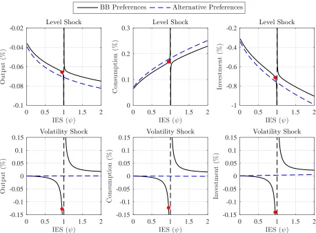
Figure 4 plots the impact effect on output, consumption, and investment from a one standard deviation increase in the level (top panels) and volatility (bottom panels) of atwith the BB

0 0.5 1 1.5 2 IES (ψ)

-0.15 -0.1 -0.05 0 0.05 0.1 0.15 O u tp u t (% ) Volatility Shock

0 0.5 1 1.5 2 IES (ψ)

-0.15 -0.1 -0.05 0 0.05 0.1 0.15 C o n su m p ti o n (% ) Volatility Shock

0 0.5 1 1.5 2 IES (ψ)

-0.15 -0.1 -0.05 0 0.05 0.1 0.15 In v es tm en t (% ) Volatility Shock

0 0.5 1 1.5 2 IES (ψ)

-0.1 -0.08 -0.06 -0.04 -0.02 O u tp u t (% ) Level Shock

0 0.5 1 1.5 2 IES (ψ)

0 0.1 0.2 0.3 C o n su m p ti o n (% ) Level Shock

0 0.5 1 1.5 2 IES (ψ)

-1 -0.8 -0.6 -0.4 -0.2 In v es tm en t (% ) Level Shock

BB Preferences Alternative Preferences

Figure 4: Impact effect on output, consumption, and investment from a1standard deviation increase in the level and volatility of the intertemporal preference shock. The circle markers show the impact when the IES is0.95(BB value).

The impact effects of the level shock are very similar for the BB preferences and our alternative specification for most values of the IES. When the household becomes more impatient, consump-tion increases and investment decreases on impact. The BB preferences show an asymptote appears in the responses of all three variables when the IES equals1, but it only has a meaningful effect on the responses if the IES is very close to1. In response to a volatility shock, the asymptote also appears when the IES equals1, but it affects the responses for a wider range of IES values. For ex-ample, there is almost no effect on output when the IES is less than0.5, whereas output decreases by about0.015%(0.025%,0.06%, 0.13%) when it equals0.7(0.8, 0.9,0.95). By setting the IES equal to0.99, the model is able to generate an enormous 0.68% decline in output. When the IES is alternatively set to1.05, output instead rises on impact by0.14%. In short, small changes in the IES lead to very different conclusions, so the model can produce any effect of demand uncertainty. The asymptote never appears with our alternative preferences, so small changes in the IES no longer significantly alter the responses to demand uncertainty shocks. There are also two key eco-nomic implications from removing the asymptote. One, the impact of a demand uncertainty shock is no longer economically significant. Output, consumption, and investment all change by less than

sav-0 0.5 1 1.5 2 IES (ψ)

-5 0 5 O u tp u t (% )

×10-4

0 0.5 1 1.5 2 IES (ψ)

-15 -10 -5 0 C o n su m p ti o n (% )

×10-4

0 0.5 1 1.5 2 IES (ψ)

0 2 4 6 8 In v es tm en t (% )

×10-3 φK = 0 φK = 2.09 φK = 4 φK= 16

(a) Impact responses as a function of the capital adjustment cost parameter (φK).

0 0.5 1 1.5 2 IES (ψ)

-2 -1 0 1 O u tp u t (% )

×10-3

0 0.5 1 1.5 2 IES (ψ)

-3 -2 -1 0 C o n su m p ti o n (% )

×10-3

0 0.5 1 1.5 2 IES (ψ)

0 2 4 6 In v es tm en t (% )

×10-3

σ= 2 σ = 80 σ = 160 σ= 1000

(b) Impact responses as a function of the coefficient of relative risk aversion (σ).

0 0.5 1 1.5 2 IES (ψ)

0 5 10 15 O u tp u t (% )

×10-4

0 0.5 1 1.5 2 IES (ψ)

-15 -10 -5 0 C o n su m p ti o n (% )

×10-4

0 0.5 1 1.5 2 IES (ψ)

0 2 4 6 8 10 In v es tm en t (% )

×10-3

φP = 0 φP = 100 φP = 200 φP = 1000

(c) Impact responses as a function of the price adjustment cost parameter (φP).

ings (reducing consumption) as well as an increase in precautionary labor supply (raising output). The above analysis compares equilibrium outcomes under the BB preferences to our alternative specification that removes the asymptote, but that exercise does not provide a complete comparison because we used the BB parameters that are chosen to fit the data conditional on their preferences. To see the range of possible predictions under our alternative preferences,figure 5shows the effect of a1standard deviation preference volatility shock as a function of the capital adjustment cost pa-rameter (φK), coefficient of relative risk aversion (σ), and price adjustment cost parameter (φP).10

In each case, a larger parameter value attenuates the counterfactual increases in output and invest-ment, especially with a larger IES. IfφK is sufficiently large, the dynamics in the model approach

those in a model with fixed capital, so investment becomes constant and output moves one-for-one with consumption. A higherσmakes households more sensitive to changes in volatility, as shown in section 3. A larger φP raises the volatility of the price markup and makes households more

sensitive to the nominal interest rate. Even with implausible values for those parameters, higher uncertainty typically raises investment, regardless of the IES. Also, the impact on output is much smaller than with the BB preferences, even with parameters that address the comovement problem.

5 P

R

This section examines potential ways to obtain larger responses to preference volatility shocks and positive comovement between output, consumption, and investment when the IES is far below1.

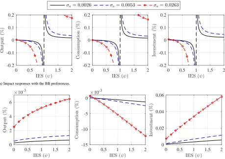
5.1 LARGERSHOCKS As shown insection 3, one way to create larger responses of real activity to a volatility shock when the IES is farther below1is by raising the steady state standard deviation of the preference shock,σa. Figure 6reproducesfigure 4with different values ofσa. With the BB

preferences, it is possible to achieve a0.13%decline in output on impact—the value BB report— whenψ is(0.95,0.90,0.67) by settingσato (0.0026,0.0053,0.0263), respectively. Thus, an IES

close to the value estimated by Smets and Wouters (2007) requires a shock standard deviation that is roughly an order of magnitude larger than the value in BB. Also, if we increase risk aversion fromσ= 80toσ = 100, double the Rotemberg price adjustment cost parameter fromφP = 100to

φP = 200, and rerun the BB impulse response matching exercise, thentable Ishows the model is

able to match both the decline in output and the volatilities in the data when the IES is0.5andσa

is doubled to0.005. With our alternative preferences the same volatility shock has very little real effect, regardless ofσa. Consistent with the discussion insection 3, we are able to reproduce the

BB results with a lower IES because larger values ofσandσawiden the influence of the asymptote.

5.2 DISASTER RISK Gourio (2012) develops a model with time-varying disaster risk, which

enters through a combination of permanent and transitory shocks to productivity and a depreciation shock to capital. According to Proposition 3 (p. 2746), if the preference shock in (1) directly hits

ut, then an increase in the probability of a disaster and a positive shock to household preferences are

observationally equivalent. In that case, the recursive structure for intertemporal utility becomes

U_tBB = [(1−β)(ad_tu(ct, nt))(1

−σ)/θ

+β(Et[(UtBB+1)1

−σ

])1/θ]θ/(1−σ)

.

The asymptote no longer appears with unit IES becausead

t revalues the current

consumption-leisure basket instead of the distributional weights. However,ad

t = (aBBt )1

−1/ψ

, so the volatility of

0 0.5 1 1.5 2 IES (ψ)

-0.2 -0.1 0 0.1 0.2

O

u

tp

u

t

(%

)

0 0.5 1 1.5 2 IES (ψ)

-0.2 -0.1 0 0.1 0.2

C

o

n

su

m

p

ti

o

n

(%

)

0 0.5 1 1.5 2 IES (ψ)

-0.2 -0.1 0 0.1 0.2

In

v

es

tm

en

t

(%

)

σa = 0.0026 σa = 0.0053 σa= 0.0263

(a) Impact responses with the BB preferences.

0 0.5 1 1.5 2 IES (ψ)

0 2 4 6

O

u

tp

u

t

(%

)

×10-3

0 0.5 1 1.5 2 IES (ψ)

-15 -10 -5 0

C

o

n

su

m

p

ti

o

n

(%

)

×10-3

0 0.5 1 1.5 2 IES (ψ)

0 0.02 0.04 0.06

In

v

es

tm

en

t

(%

)

(b) Impact responses with our alternative preferences.

Figure 6: Impact effect on output, consumption, and investment from a 1 standard deviation preference volatility shock. All of the parameters except the IES and preference shock standard deviation are set to the values in BB.

Unconditional Volatility Stochastic Volatility

Moment Data Larger Shock Disaster Risk Data Larger Shock Disaster Risk

Output 1.1 0.9 1.1 0.4 0.2 0.2

Consumption 0.7 0.7 0.7 0.2 0.1 0.1

Investment 3.8 4.7 4.7 1.6 1.0 0.9

Table I: Standard deviations with the BB preferences (%). The data sample is 1986-2014. The model-based statistics reflect the average from repeated simulations with the same length as the data. Stochastic volatility is measured by the standard deviation of the time-series of 5-year rolling standard deviations. These procedures follow table 2 from BB.

ad

t is much larger whenψ is near zero.11 Therefore, we reran the BB impulse response matching

exercise with the IES set to 0.05. As table I shows, we were able to restore the BB results with disaster risk preferences. However, with such a low IES, we had to more than double the risk-aversion parameter from80to200and triple the Rotemberg price adjustment cost parameter from

100to300. The algorithm also increased the capital adjustment cost parameter from2.09to9.86.

11_{Also, the disaster risk specification is not observationally equivalent to the preference shock specification in the}

0 0.5 1 1.5 2 IES (ψ)

-0.2 -0.15 -0.1 -0.05 0

Output (%)

0 0.5 1 1.5 2 IES (ψ)

-0.2 -0.15 -0.1 -0.05 0

Consumption (%)

0 0.5 1 1.5 2 IES (ψ)

-0.2 -0.15 -0.1 -0.05 0

Investment (%)

Figure 7: Impact effect on output, consumption, and investment from a1standard deviation preference volatility shock under the disaster risk preferences. The circle markers show the impact effect when the IES equals0.05—a value that achieves similar responses as the original BB specification. All other parameters are re-estimated with the BB method.

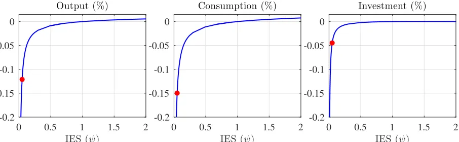
To get a broader sense of how the IES affects the response of real activity,figure 7reproduces

figure 4with disaster risk preferences. There are two key points. One, the responses are continuous for positive IES values, so there is no longer a discrete jump in the impact effect at unit IES. However, the predictions of the model are still very sensitive to the IES. For example, doubling the IES from 0.05to 0.1causes the impact effect on output to decline from 0.12% to0.06%, and an IES of0.5causes output to decrease less than0.01%. The sensitivity to the IES is similar to what we reported with the BB preferences. Two, there is no economic effect at unit IES, as stressed by Gourio (2012). Therefore, the responses to a volatility shock are quite different from the BB preferences, which generated the largest effects of volatility shocks when the IES was near unity.12

6 C

Since the financial crisis, aggregate demand shocks driven by changes in intertemporal preferences have become commonplace in macroeconomists’ toolkits. Intertemporal uncertainty shocks in combination with recursive preferences are much less common. Our paper highlights that the novel findings in BB rest on an—until now—undetected asymptote. We suggest a simple alternative specification that removes the asymptote and provides predictions that are robust to small changes in the IES. Under this specification, preference volatility shocks have negligible effects on macro aggregates for plausible parameterizations. The question is whether it is possible to rationalize the asymptote. Providing an axiomatic account of the BB preferences is beyond the scope of this paper. However, we point out two puzzling features. The covariance between the preference shock and the value function changes sign at an IES of 1 and it is very large when the IES is near 1, so small changes in relative discounting have big effects on the level of utility.13 _{Therefore, we} believe the uncertainty puzzle—why models struggle to generate sizeable movements in economic activity in response to changes in uncertainty, in contrast to the empirical evidence—remains.

12_{Another alternative is a risk premium volatility shock, which creates positive comovement between consumption} and investment and thus slightly larger responses than a preference volatility shock with our alternative preferences.

R

ALBUQUERQUE, R., M. EICHENBAUM, V. X. LUO, AND S. REBELO (2016): “Valuation Risk and Asset Pricing,” The Journal of Finance, 71, 2861–2904.

BACHMANN, R., S. ELSTNER, AND E. SIMS(2013): “Uncertainty and Economic Activity: Evi-dence from Business Survey Data,” American Economic Journal: Macroeconomics, 5, 217–49. BANSAL, R. AND A. YARON (2004): “Risks for the Long Run: A Potential Resolution of Asset

Pricing Puzzles,” The Journal of Finance, 59, 1481–1509.

BASU, S. AND B. BUNDICK (2017): “Uncertainty Shocks in a Model of Effective Demand,” Econometrica, 85, 937–958.

BASU, S.ANDM. KIMBALL(2002): “Long-Run Labor Supply and the Elasticity of Intertemporal Substitution for Consumption,” Manuscript, University of Michigan.

BLOOM, N. (2009): “The Impact of Uncertainty Shocks,” Econometrica, 77, 623–685.

BORN, B. AND J. PFEIFER (2014): “Policy Risk and the Business Cycle,” Journal of Monetary Economics, 68, 68–85.

EPSTEIN, L. G.ANDS. E. ZIN (1991): “Substitution, Risk Aversion, and the Temporal Behavior of Consumption and Asset Returns: An Empirical Analysis,” Journal of Political Economy, 99, 263–86.

FERNANDEZ-VILLAVERDE, J., P. GUERR´ ON-QUINTANA, K. KUESTER,´ AND J. F. RUBIO-RAM´IREZ (2015): “Fiscal Volatility Shocks and Economic Activity,” American Economic Re-view, 105, 3352–84.

FERNANDEZ-VILLAVERDE, J., P. GUERR´ ON-QUINTANA, J. F. RUBIO-RAM´´ IREZ, AND M. URIBE (2011): “Risk Matters: The Real Effects of Volatility Shocks,” American Economic Review, 101, 2530–61.

GOURIO, F. (2012): “Disaster Risk and Business Cycles,” American Economic Review, 102, 2734–2766.

HALL, R. E. (1988): “Intertemporal Substitution in Consumption,” Journal of Political Economy, 96, 339–357.

HANSEN, L. P. AND T. J. SARGENT (2008): Robustness, Princeton, NJ: Princeton University Press.

JUSTINIANO, A.ANDG. E. PRIMICERI (2008): “The Time-Varying Volatility of Macroeconomic Fluctuations,” American Economic Review, 98, 604–41.

KOLLMANN, R. (2016): “International business cycles and risk sharing with uncertainty shocks and recursive preferences,” Journal of Economic Dynamics and Control, 72, 115–124.

MUMTAZ, H.ANDF. ZANETTI(2013): “The Impact of the Volatility of Monetary Policy Shocks,” Journal of Money, Credit and Banking, 45, 535–558.

RICHTER, A. W. AND N. A. THROCKMORTON (2017): “A New Way to Quantify the Effect of Uncertainty,” Federal Reserve Bank of Dallas Working Paper 1705.

RUDEBUSCH, G.AND E. SWANSON (2012): “The Bond Premium in a DSGE Model with Long-Run Real and Nominal Risks,” American Economic Journal: Macroeconomics, 4, 105–43. SMETS, F. ANDR. WOUTERS(2007): “Shocks and Frictions in US Business Cycles: A Bayesian

DSGE Approach,” American Economic Review, 97, 586–606.