Working from home and the willingness to accept a longer commute

https://doi.org/10.1007/s00168-018-0873-6

O R I G I N A L P A P E R

Working from home and the willingness to accept a longer

commute

Duco de Vos1 ·Evert Meijers1 ·Maarten van Ham1,2

Received: 27 June 2017 / Accepted: 25 June 2018 © The Author(s) 2018

Abstract

It is generally found that workers are more inclined to accept a job that is located farther away from home if they have the ability to work from home one day a week or more (telecommuting). Such findings inform us about the effectiveness of telecommuting policies that try to alleviate congestion and transport-related emissions, but they also stress that the geography of labour markets is changing due to information technology. We argue that estimates of the effect of working from home on commuting time may be biased because of sorting based on residential- and commuting preferences. In this paper we investigate the relationship between telecommuting and commuting time, controlling for preference-based sorting. We use 7 waves of data from the Dutch Labour Supply Panel and show that on average telecommuters have higher marginal cost of one-way commuting time, compared to non-telecommuters. We estimate the effect of telecommuting on commuting time using a fixed effects approach, and we show that preference-based sorting biases cross-sectional results upwards. This suggests that the bias due to sorting based on residential preferences is strongest. Working from home allows people to accept 5% longer commuting times on average, and every additional 8 h of working from home are associated with 3.5% longer commuting times.

JEL Classification R11·R41·J32

1 Introduction

There is an ongoing debate about the extent to which working from home (also called telecommuting) affects the length of the commute people are willing to accept. Early

B

1 _{Faculty of Architecture and the Built Environment, Delft University of Technology, Julianalaan}

134, 2628 BL Delft, Netherlands

2 _{School of Geography and Geosciences, University of St Andrews, Irvine Building,}

interest in the effect of telecommuting on commuting distance and household travel was mainly aimed at establishing whether telecommuting could be an effective policy instrument to alleviate congestion and emissions associated with car use (Salomon

1985; Nilles1991; Lund and Mokhtarian1994). Increasingly, attention is being given to the notion that telecommuting also affects the geography of labour markets, for example, by having a positive effect on job accessibility (Muhammad et al. 2008; Van Wee et al.2013). Understanding the relationship between telecommuting and the length of the commute may thus both inform policies aimed at alleviating conges-tion and transport-related emissions, and policies that aim to improve the economic performance of cities and regions.

Most empirical work on the effects of working from home on commuting tends to corroborate the intuitive notion that being able to avoid the commute one day in the week makes workers more willing to accept a longer commute on the other days of the week (Jiang2008; Zhu2012; Kim et al.2015). However, estimates for the size of this effect vary across the literature, the set of control variables included differs between studies, and there is little attention for the intensity of telecommuting (the number of days per week/month). Moreover, there is no consensus on a strategy to deal with sources of bias stemming from the fact that commute length and telecommuting are often decided upon simultaneously. While some studies aim to eliminate the positive bias that arises if long commutes influence the decision to telecommute (Jiang2008; Zhu2012), there is a lack of attention for preference-based sorting. OLS estimates will be biased downward if workers who dislike commuting, and hence have shorter commutes, might also be more likely to work from home. On the other hand, those who have long commutes may be the ones that value residing in more rural areas, where housing quality is cheaper, and working from home may also be more attractive. The latter type of sorting would bias OLS estimates upward.

2 Telecommuting and the length of the commute

2.1 Theoretical implications of telecommuting

The potential spatial effects of telecommuting and other ICT activities have been theorized upon for at least 50 years. According to Webber (1963), the observed spatial expansion of market areas during the 1960s due to, inter alia, information flows was indicative of a looming “demise of the city” (Webber1963, p. 1099). Such visions were generally based on the idea that information and communications technology would eventually substitute face-to-face contact, and have been a recurrent theme in futurist writings on the death of cities, and the death of distance (Toffler1980; Naisbitt

1994; Cairncross1997).

In much of the literature, telecommuting is seen as a potential policy instrument to decrease car travel, of which the effectiveness is dependent on the overall effect on travel. In transportation research it is often stressed that telecommuting, and ICT activi-ties in general, may substitute, complement, modify, or neutrally affect travel (Salomon

1985). The notion of complementary travel is based on the idea that telecommuting may induce people to accept jobs over longer distances, making the net travel effects of telecommuting not necessarily negative. Furthermore, it is argued that households have a rather fixed mobility budget, and a decrease in trips for commuting would be substituted by leisure trips, and trips of other household members (De Graaff2004).

However, the welfare effects of telecommuting may stretch further, because work-ers that are able to telecommute can expand the geographical areas in which they look for jobs (Van Wee et al.2013). Basic urban economic models support the intuition that if telecommuters have less commuting trips than non-telecommuters, they bid less for homes closer to the Central Business District (the location of employment), and more for suburban homes (Alonso1974; Lund and Mokhtarian1994; Jiang2008). Rhee (2008) shows that in theory, similar results could be obtained in cities with dispersed employment. In situations with little building restrictions, telecommuting may thus in theory promote residential sprawl in a similar way as the automobile did (Glaeser and Kahn2004). In settings with strict urban containment policies, and a low elasticity of housing supply, such as the Netherlands (Vermeulen and Rouwendal2007), possibili-ties for telecommuting may increasingly enable workers to live in one city and reap the benefits of access to labour in other cities (Muhammad et al.2008; Van Wee et al.2013). In the current work we are predominantly interested in the effect of telecommuting on the geographical scale of labour market areas. Therefore, we focus on the relatively uncontested mechanism by which telecommuting potentially increases the length of one-way commutes, because it allows workers to commute less frequently. We do not take into account the effects of telecommuting on non-commute trips, and travel behaviour of other household members.

2.2 Empirical issues

commodity. In a seminal publication, Nilles (1991) investigates the potential effects of telecommuting on urban sprawl and household travel, using data from a telecommuting experiment with California State workers that spanned 2 years. He concludes that at the time, telecommuting did not (yet) exacerbate urban sprawl, and that it resulted in decreased household travel. He did, however, find that telecommuting was associated with moves farther away from the work location, so his findings did not rule out future

telesprawlas a consequence.

Later evidence on the relationship between telecommuting and the length of the commute is somewhat scattered, in part because of different definitions of telecom-muting.1In a review of evidence by De Graaff (2004) it is concluded that most studies show a negative relationship between telecommuting and the number of commuting trips, and studies that do investigate the length of the commute find mixed evidence, but do not rule out a positive relationship. Andreev et al. (2010) conclude similarly, and stress that the majority of the literature suffers from problems such as the lack of a universal definition of telecommuting, the external validity of the results, and the absence of theoretical substantiation of the results.

Recent endeavours increasingly pay attention to potential sources of bias that influence the results from observational studies. These sources can be divided into (1) omitted variables, (2) reverse causality, and (3) preference-based sorting. With respect to omitted variables, the advent of large-scale surveys in which questions about telecommuting were asked, made it possible to control for a variety of respon-dent characteristics, and also made it possible to assess telecommuting across different industries. A notable work in this respect is Kim et al. (2012), who estimated the effect of telecommuting on peripheral living, controlling extensively for household charac-teristics including income, and job locations. Accounting for wage seems particularly relevant in telecommuting research, because earnings and telecommuting status tend to be correlated (Muhammad et al.2008).

Jiang (2008, p. 10) provides a clear-cut definition of two other types of bias involved in the relationship between telecommuting and commuting distance, and the direction of these biases: “If [a] longer commute encourages an individual to work from home when allowed, a regression of commute length on telecommuting status will overesti-mate the effect of telecommuting. On the contrary, telecommuters could be those who feel more pressures from traffic. They would have shorter commutes in the absence of telecommuting opportunities. This unobserved selection will lead to a downward [bias] in the regression estimates”. We refer to the first bias he addresses as reverse causality, and to the second as sorting based on commuting preferences.

Commuting time and telecommuting may not only be jointly influenced by com-muting preferences, but also by residential preferences. Individuals that prefer rural living, and generally have longer commutes, may have larger or more comfortable houses because housing quality tends to be cheaper away from central business areas (Muth1969). Assuming that spending time in higher quality housing is more plea-surable than spending time in houses of lower quality (Gubins and Verhoef2014), we may expect that working from home is more attractive for rural dwellers. With

1 _{Mokhtarian et al. (2005) illustrate that definitions, measurement instruments, sampling, and vested}

this type of sorting based on residential preferences, an OLS regression of commuting time on telecommuting status would overestimate the real relationship.

A study in which an attempt is made to overcome the bias from potential reverse causality is done by Zhu (2012). He employs an instrumental variables approach, using the number of phones in a household, and the usage of the internet at home as instruments, argued to influence commuting distance only through the effects on telecommuting. Although the reverse causality bias he refers to should lead to overes-timation of the effect of telecommuting, he finds that his IV approach leads tohigher estimates, compared to OLS. According to his IV results for the year 2009, telecom-muters that work from home at least once a week have a 1576% longer commuting distance, and a 160% longer commuting duration on average.2While these estimates are large, the results suggest that the bias not accounted for in OLS models is positive rather than negative.

Jiang (2008) uses a similar IV approach, but the instruments in this study are based on the penetration of home-based teleworking across combinations of occupations and city size classes. The results of this study show that OLS tends to underestimate the real effect of telecommuting. While the OLS estimates in this study show that, at least for married women, telecommuting increases commuting time by 3 min, the IV estimates suggest an effect of 9–11 min. No significant results are found for men, and single women.

The current study addresses several gaps that emerge from the literature. First, next to household characteristics we include detailed job characteristics as control variables, including monthly wage, the type of industry, the type of employment, and the usual number of work days per week. Especially the latter control is a novelty in this type of research. Second, we make use of the time dimension of our data, and we focus on the effect ofchangesin telecommuting status, onchangesin commuting time.3Arguably, this makes the potential bias of reverse causality less pressing. While exogenous changes in commuting time (for instance due to firm relocations) may influence the decision to telecommute, this still indicates that telecommuting increases the willingness to accept a longer commute. Finally, the time dimension of the data also allows us to control for all time-invariant characteristics of respondents through the use of fixed effects models. Such time-invariant characteristics include unobserved commuting- and residential preferences, so this approach allows us to address the bias due to preference-based sorting. This is one of the first studies to address the relationship between telecommuting and commuting distance with a fixed effects approach.4

2 _{Given his log-linear model, these are the marginal effects of the telecommuting dummy for which the}

point estimate is 2.819 for the distance model, and 0.993 for the duration model. The marginal effects are calculated as (eβ−1)∗100%. The corresponding marginal effects of his OLS estimates are more realistic: 23 and 19%, respectively.

3 _{The fixed effects models use variation in telecommutingwithinindividuals, over time, to explain}

time-variation in commuting time within individuals.

4 _{Two notable studies that apply a fixed effects to approach to telecommuting research are De Graaff}

3 Data and methods

3.1 Data description

Our empirical analyses are based on data from the Netherlands. The urban landscape of the Netherlands is characterized by a polycentric urban structure with many small-and medium-sized cities. Labour- small-and housing markets stretch far beyond cities, small-and it is relatively common to live in or near one city, and work in another urban area (Burger and Meijers2016). Another notable characteristic is the concentration of employment in the Randstad area, in the west of the country. This area is also characterized by a higher wage level (Groot et al.2014), and better matching between workers and employers indicated by lower levels of overeducation (Büchel and Van Ham2003). In the Netherlands telecommuting is a relatively widespread phenomenon, due to the mass adoption of ICT, the high share of the tertiary sector in economic activities, and the high population density and the associated congestion problems (Muhammad et al.2007,2008).

The data we use come from the Labour Supply Panel (SCP2016), and it consists of the 7 latest biannual waves (between 2002 and 2014). While the panel has been running since 1985, 2002 is the first year in which questions were asked about the degree to which people work from home. We have 18,730 observations for 7497 individuals.5

3.2 Telecommuting definition

We are interested in the relationship between telecommuting and the (accepted) com-muting time. As mentioned earlier, a variety of definitions of telecomcom-muting is used in related literature. Mokhtarian et al. (2005) give an overview, starting from the idea that telecommuting involves “salaried employees of an organization [that] replace or modify the commute by working at home or a location closer to home than the regular workplace, generally using ICT […]” (Mokhtarian et al.2005, p. 427). Studies from their literature review have threshold values for the intensity of telecommuting that range from at least once per month, to at least once per week.

Two questions from the survey we use relate to the intensity of telecommuting. The first asks to state how many days per month respondents work from home usually. The answers to this question are measured on an ordinal scale with 5 possibilities (0, 1, 2, and 3 days, and more than 3 days). The second question asks to state the average number of weekly hours spent from home in the 4 weeks before the survey date, and the resulting variable is measured on a continuous scale. Both questions contain some ambiguities, the first one about what is meant by “usually” and the second one about whether these hours working from home substitute commuting activities. Therefore, our definition of telecommuters will be based on workers who usually work at home

5 _{We excluded extreme observations with commuting times longer than 500 min, monthly wages lower}

.1

.15

.2

.25

2002 2004 2006 2008 2010 2012 2014 Year

Share telecommuters

1.5

2

2.5

3

3.5

2002 2004 2006 2008 2010 2012 2014 Year

Hours telecommuting

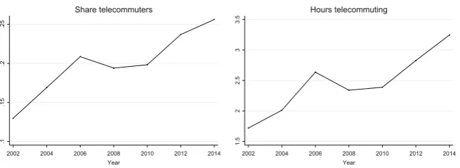
Fig. 1Time patterns of working from home

at least once per month, and have worked from home at least 4 h on average during the 4 weeks before the survey date.6

Another question asks whether respondents use email or internet to work from home. Limiting our sample to salaried employees, our data thus allow us to define telecommuting as workers who work regularlyfrom home, substituting commuting activities, and using ICT. The only discrepancy with the definition of Mokhtarian et al. (2005) involves workers who telecommute from a location closer to home than the regular workplace. To the extent that we still measure telecommuting with an error, our estimates will be biased towards zero.

We will perform our analyses using (1) a dummy that indicates whether or not a respondent telecommutes, (2) an ordinal factor variable that denotes the usual number of telecommuting days per month, and (3) a continuous measure of the average weekly hours working from home (for telecommuters). Figure 1 shows the time patterns of the share of telecommuters, and the average weekly hours working from home. Both graphs show an increase in telecommuting (intensity) between 2002 and 2014, with a dip in the years 2008 and 2010.7The overall increasing pattern stresses that telecommuting is still a dynamic and upcoming trend.

3.3 Other variables and summary statistics

Commuting time is measured as the usual time it takes to get to work from the residen-tial location. The data does not contain information on commuting distance. However, modelling commuting distance is generally plagued by assumptions about mode choice and commuting speed (Isacsson et al.2013), while the use of commuting time can be justified by the assumption that commuting speed is optimally chosen (Van Ommeren and Fosgerau2009).

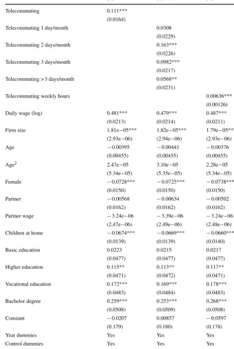
Figure 2 shows the (kernel) distribution of one-way commuting time for non-telecommuters, occasional telecommuters (up to 3 days per month), and regular

6 _{The 4 h on average per week are chosen to come close to a threshold value of 2 telecommuting days per}

month, which holds the middle ground between the threshold values mentioned in Mokhtarian et al (2005).

7 _{Data from the US Community Survey show a similar dip in working from home around 2008, and in the}

0

.01

.02

.03

Kernel density

0 50 100 150 200

Minutes

No telecommuting

Telecommuting 1-3 days/month Telecommuting > 3 days/month

Commuting time

Fig. 2Distribution of commuting time according to telecommuting status. The density functions are esti-mated with a Gaussian kernel, and a bandwidth of 5 min

Table 1Telecommuting and

changes in commuting time N Mean change SD

Started telecommuting betweent−2 andt

975 1.494 17.358

No change 9554 0.307 14.377 Quit telecommuting

betweent−2 andt

704 −0.652 19.885

telecommuters (more than 3 days per month). The figure shows that the distribution of commuting times for non-telecommuters has its bulk between 0 and 25 min, while the distributions of the other categories are more spread, including relatively longer com-mutes. The average commuting time for non-telecommuters is 24 min, versus 32 min for occasional telecommuters, and 31 min for regular telecommuters. So far, it seems that non-telecommuters have considerably shorter commutes on average, while regular telecommuters do not have longer commuting times than occasional telecommuters.

In Table1we make use of the time dimension of our data, and a similar pattern emerges. Commuting times of respondents who started to telecommute between two consecutive waves increased by 1.5 min on average, while the average increase is 0.31 for respondents for whom nothing changed, and average commuting times decreased for respondents that quit telecommuting.8

Other essential variables are all deduced from answers to questions in the survey: we calculate the daily wage of respondents based on the (stated) net wage per month and the usual number of working days per week, assuming 6 weeks of vacation on average; job search is measured as a dummy indicating the respondent is searching for a job at the moment the survey was conducted; job mobility is measured as a dummy that indicates whether or not the respondent changed jobs between two consecutive survey waves, and in our analysis we use the 2-year lead of this variable.

Table2shows the summary statistics of variables used in our analyses, including the average number of working days per week, firm sector and size, age, sex, the presence of children and a partner, and the wage of the partner.

3.4 Methods

We introduced two types of preference-based sorting that may bias OLS results: sort-ing based on commutsort-ing preferences and sortsort-ing based on residential preferences. Our data allow us to investigate whether commuting preferences significantly differ between telecommuters and non-telecommuters. In the first part of our empirical anal-ysis therefore, we use a model based on job search theory to calculate the marginal monetary value of one-way commuting time (MCC) both for both groups separately. If the MCC is significantly higher for telecommuters, we interpret this as evidence for sorting based on commuting preferences.

Using the job search approach we relate commuting time and wage levels with each other through their effects on (1) on-the-job search, and (2) job mobility (Van Ommeren and Fosgerau2009). The intuition behind this approach is that workers are not in their preferred job per se, and are able to improve upon their situation by searching for jobs, and moving jobs if they find a better fit that improves theirlifetime utility (Van Ommeren et al.2000). By calculating the effect of commuting time on job search and job moving, we get an indication of the willingness to accept longer commuting times. Moreover, by calculating the ratio of the effect of commuting time and the effect of wages, we can put a monetary value on this willingness to accept (Van Ommeren and Fosgerau2009). The advantage of this approach is that we do not need to assume that labour markets are in equilibrium (Gronberg and Reed1994). In other words, we do not need to assume that observed situations in the labour market reflect the best choices among all available alternatives.

Conceptually, our regression model distinguishes between telecommuting as a job asset, and telecommuting as a substitute for commuting physically. We investigate the effect of telecommuting on the acceptability of one-way commuting times by examining the interactions between a telecommuting dummy and commuting distance. The main effect of this telecommuting dummy tells us something about the intrinsic value of telecommuting. Several studies suggest for instance that working from home on designated, individual tasks may increase worker productivity (Bernardino2017). Furthermore, the possibility to telecommute may increase the chance of matching between workers and employers if labour markets for telecommuting jobs indeed have a larger geographical scale.

Table 2Summary statistics of full sample

Variables N Mean SD Min. Max.

Telecommuting 18,730 0.2 0.4 0 1

Telecommuting 0 days/month 18,730 0.681 0.466 0 1

Telecommuting 1 day/month 18,730 0.0984 0.298 0 1 Telecommuting 2 days/month 18,730 0.0758 0.265 0 1

Telecommuting 3 days/month 18,730 0.0753 0.264 0 1

Telecommuting > 3 days/month

18,730 0.0698 0.255 0 1

Telecommuting weekly hours 18,730 2.467 6.803 0 97

Commuting time 18,730 26.81 21.07 0 180

Job search at t 18,730 0.114 0.317 0 1 Job move betweent−2 andt 18,730 0.154 0.361 0 1

Job move betweentandt+ 2 11,320 0.104 0.306 0 1

Daily wage 18,730 106.5 44.76 21.06 808.7

Monthly wage 18,730 1.742 791.9 501 16,667 Working days/week 18,730 4.323 0.965 1 7

Firm size 18,730 613.2 2.446 0 70,000

Age 18,730 43.11 11.04 16 66

Female 18,730 0.468 0.499 0 1

Partner 18,730 0.798 0.402 0 1

Partner wage 18,730 1.148 2.567 0 75,000 Children at home 18,730 0.571 0.495 0 1

Primary education 18,730 0.0153 0.123 0 1

Basic education 18,730 0.189 0.392 0 1 Higher education 18,730 0.38 0.485 0 1

Vocational education 18,730 0.29 0.454 0 1

Bachelor degree 18,730 0.125 0.331 0 1 Sector: agriculture 18,730 0.00769 0.0873 0 1

Sector: industry 18,730 0.122 0.327 0 1

Sector: construction 18,730 0.041 0.198 0 1 Sector: trade 18,730 0.122 0.328 0 1

Sector: transport 18,730 0.0569 0.232 0 1

Sector: business services 18,730 0.178 0.382 0 1 Sector: healthcare 18,730 0.204 0.403 0 1

Sector: other 18,730 0.0456 0.209 0 1

Sector: government 18,730 0.107 0.309 0 1 Sector: education 18,730 0.117 0.321 0 1

Job type: civil servant 18,730 0.191 0.393 0 1

Job type: employee 18,730 0.8 0.4 0 1

0

.05

.1

.15

.2

0-20 20-40 40-60 >60 Commuting time

Job search

0

.05

.1

.15

0-20 20-40 40-60 >60 Commuting time

Job change (t+2)

Fig. 3Bivariate relationships between commuting time and job search (l), and job mobility (r)

4 Results

4.1 Evidence for preference-based sorting

In this subsection we examine the difference in commuting preferences between telecommuters and non-telecommuters. We do this by estimating the effect of com-muting time on job search and the propensity to change jobs, for both groups. We standardize this effect by the effects of wage on job search and mobility to obtain the marginal costs of one-way commuting time (MCC), measured as the average amount of daily wage people are willing to give up to shorten their (one-way) commute with 1 min (Van Ommeren and Fosgerau2009). First, in Fig.3we show the bivariate rela-tionship between commuting time and job search and mobility for the whole sample. It is clear that both the share of people looking for a job and the share of people chang-ing jobs within 2 years are positively related with commutchang-ing time. This confirms the intuitive notion that longer commutes are seen as a negative aspect of jobs.9

In Table3we estimate the daily MCC using the two distinct approaches. We follow the literature and use a random effects probit model to deal with potential heterogene-ity among different individuals.10 According to the job search model in column (1) commuting time has a greater effect on job search for telecommuters than for non-telecommuters. In monetary terms, non-telecommuters are willing to accept a 1 min longer one-way commute fore2.63 per work day, while telecommuters are willing to accept a 1 min longer commute fore3.80.11Note that this is in spite of the fact that, by definition, telecommuters commute less frequently, compared to non-telecommuters, so the MCC per commuting trip may be even higher for telecommuters. Furthermore, according to this model age has a positive but marginally decreasing effect on the propensity to search, and higher educated people search more. The effect of telecom-muting itself is insignificant.

In column (2) we estimate the same model with job mobility (changing jobs within 2 years) as the dependent variable. According to this model the MCC ise1.91 for

9 _{We found no such clear bivariate patterns between telecommuting and job search and mobility.} 10 _{This allows the error terms of the same individuals to be correlated over time (Van Ommeren and}

Fosgerau2009).

Table 3Willingness to pay for commuting regressions

(1) (2)

Job search Job mobility

Commute * no telecommuting 0.00494*** 0.00330***

(0.000927) (0.00117)

Commute * telecommuting 0.00712*** 0.00372** (0.00128) (0.00155)

Telecommuting −0.0597 0.112

(0.0671) (0.0824)

Daily wage −0.00187*** −0.00172**

(0.000545) (0.000787)

Firm size 4.75e−06 −2.89e−05

(6.12e−06) (1.77e−05)

Age 0.0755*** −0.0320*

(0.0131) (0.0170)

Age2 −0.00114*** 3.01e−05

(0.000157) (0.000207)

Female 0.0263 −0.0954*

(0.0441) (0.0570)

Partner −0.217*** −0.177***

(0.0475) (0.0610)

Partner wage −5.59e−06 1.58e−05** (6.71e−06) (6.96e−06)

Children at home 0.0130 0.0329

(0.0424) (0.0533)

Basic education −0.0764 −0.0290

(0.152) (0.160)

Higher education 0.0201 0.00369

(0.151) (0.158)

Vocational education 0.279* 0.166

(0.154) (0.162)

Bachelor degree 0.449*** 0.210

(0.160) (0.172)

Constant −1.841*** 0.703

(0.389) (0.567)

Individual random effects Yes Yes

Year dummies Yes Yes

Control dummies Yes Yes

Observations 18,730 11,320

Individuals 7497 4481

Table 3continued

(1) (2)

Job search Job mobility

Log likelihood −6136 −3493

MCC non-telecommuters e2.63 e1.91

MCC telecommuters e3.80 e2.15

Relative difference 1.44 1.13

Robust std. errors in parentheses. Control dummies include 7 working days-, 10 industry-, and 5 job type dummies. MCC stands for marginal cost of commuting, and should be interpreted as the daily willingness-to-pay for a 1 min reduction in one-way commuting time

***p< 0.01; **p< 0.05; *p< 0.1

non-telecommuters, ande2.15 for telecommuters. These values are lower than the estimates in the previous model. The ratio between these values is also lower (1.13 vs. 1.44). According to this model the effect of age on mobility is predominantly negative, and higher educated people seem more mobile, but not significantly so. The effect of telecommuting itself on job moving is not significant.

In conclusion, this part of the analysis shows that the MCC is between 13 and 44% higher on average for telecommuters, in spite of the fact that their commut-ing frequency is lower. Therefore, it is established that preferences of telecommuters differ significantly from non-telecommuters in terms of commuting tolerance. More specifically, if there was only sorting based on commuting preferences, not taking into account these preferences when analyzing the effect of telecommuting on commut-ing time would lead to underestimation of the real effect. We find no evidence that telecommuting is a positive job asset in itself.

4.2 Commuting time

In this subsection we estimate the effect of telecommuting on commuting time, con-trolling for preference-based sorting by employing individual fixed effects. We start with an OLS model, and we compare the resulting estimates with the results of a fixed effects model. Because the dependent variable is in logs, 187 observations with 0 com-muting time are excluded from the analysis, so we are left with 18,543 observations. Table4shows the OLS results. In column (1) we use a telecommuting dummy that corresponds to our telecommuting definition. According to this model telecommuting results in a 11.7% longer commute on average.12Furthermore, a 10% increase in daily wage is associated with a 4.8% increase in commuting time, the level of education has a positive effect on commuting time, commuting patterns are gendered (women have about 7.6% shorter commutes), and individuals with children at home have about 7% shorter commutes. Except for the insignificant effect of age, these findings are in line with earlier results on Dutch commuting behaviour, which showed that females, and people with children, have shorter commutes on average, and people of higher

socio-12 _{The coefficients in these log-linear models should be interpreted as an (e}β_{−1)∗100% increase for}

Table 4OLS commuting time regressions

(1) (2) (3)

Telecommuting 0.111***

(0.0164)

Telecommuting 1 day/month 0.0308 (0.0229)

Telecommuting 2 days/month 0.163***

(0.0226) Telecommuting 3 days/month 0.0982***

(0.0217)

Telecommuting > 3 days/month 0.0568** (0.0231)

Telecommuting weekly hours 0.00636***

(0.00126) Daily wage (log) 0.481*** 0.479*** 0.487***

(0.0213) (0.0214) (0.0211)

Firm size 1.81e−05*** 1.82e−05*** 1.79e−05*** (2.93e−06) (2.94e−06) (2.93e−06)

Age −0.00395 −0.00441 −0.00376

(0.00455) (0.00455) (0.00455)

Age2 2.47e−05 3.10e−05 2.28e−05 (5.34e−05) (5.35e−05) (5.34e−05)

Female −0.0728*** −0.0725*** −0.0738***

(0.0150) (0.0150) (0.0150) Partner −0.00568 −0.00634 −0.00502

(0.0162) (0.0162) (0.0162)

Partner wage −3.24e−06 −3.39e−06 −3.24e−06 (2.47e−06) (2.49e−06) (2.48e−06)

Children at home −0.0674*** −0.0669*** −0.0660***

(0.0139) (0.0139) (0.0140) Basic education 0.0223 0.0215 0.0217

(0.0477) (0.0477) (0.0477)

Higher education 0.115** 0.113** 0.117** (0.0471) (0.0472) (0.0471)

Vocational education 0.172*** 0.169*** 0.178***

(0.0483) (0.0484) (0.0483) Bachelor degree 0.259*** 0.253*** 0.268***

(0.0508) (0.0509) (0.0508)

Constant −0.0207 0.00857 −0.0597

(0.179) (0.180) (0.178)

Year dummies Yes Yes Yes

Table 4continued

(1) (2) (3)

Observations 18,543 18,543 18,543

R-squared 0.132 0.132 0.132

Dependent variable: commuting time (log). Robust std. errors in parentheses. In columns (1) and (2) no telecommuting is the reference category. Control dummies include 7 working days-, 10 industry-, and 5 job type dummies

***p< 0.01; **p< 0.05; *p< 0.1

economic status commute longer (Van Ham2002; Burger et al.2014). Employees of larger firms commute longer according to this model.

In column (2) we distinguish between 1, 2, 3, and more than 3 days of telecommuting per month. The results show that the positive effect found in the previous column is mainly driven by telecommuters that telecommute 2–4 days per month, as the effect of telecommuting 1 day per month is small and insignificant. The coefficients of the other variables are virtually unaffected by this alternative measure of telecommuting. In column (3) we measure telecommuting by the usual number of hours per week spent telecommuting. Arguably this is the most precise measure of telecommuting intensity. According to the model every 8 additional hours of telecommuting lead to a 5.2% increase in commuting time. The other coefficients are again similar to those in previous models.

In Table5we estimate the same models including individual specific fixed effects that correct for all time-invariant attributes of individuals, including preferences. Coef-ficients are estimated based on variationwithinindividuals over time. The results from column (1) indicate that telecommuting leads to 5% longer commutes, rather than the 11.7% estimated in column one. Thus, the extent of the bias due to sorting is positive (+ 128%) according to this specification. The fixed effects model results in several different coefficients compared to the OLS estimates. First, the effect of daily wage on commuting time is lower when accounting for time-invariant unobservables. This may for instance be driven by correlations between capability and labour mobility. Second, it seems that ageing does not significantly influence commuting time. Third, changes in firm size and having children at home have significant but smaller effects on commuting time, compared to the OLS model. Finally, while we see an increasing pattern in the effects of education on commuting, the estimates are not significant.

Column (2) is the fixed effects equivalent of Table4, column (2). The results from this column show that compared to non-telecommuters, individuals that telecommute 1 day per month accept a 6.1% longer commute, those telecommuting 2 days per month a similar but lower 5.1%, those that telecommute 3 days do not have significantly longer commutes. This result is somewhat counter-intuitive as it suggests positive but decreasing effect of telecommuting on commuting time. It should, however, be noted that the only significant difference in coefficients betweenconsecutivecategories is the one between no telecommuting and telecommuting 1 day per month. Other coefficients in this model are similar to those in the previous column.

Table 5FE commuting time regressions

(1) (2) (3)

Telecommuting 0.0486***

(0.0141)

Telecommuting 1 day/month 0.0590*** (0.0187)

Telecommuting 2 days/month 0.0494***

(0.0189) Telecommuting 3 days/month 0.0290

(0.0186)

Telecommuting > 3 days/month 0.000951 (0.0185)

Telecommuting weekly hours 0.00425***

(0.000827) Daily wage (log) 0.176*** 0.176*** 0.176***

(0.0270) (0.0270) (0.0269)

Firm size 5.36e−06** 5.37e−06** 5.28e−06** (2.13e−06) (2.13e−06) (2.13e−06)

Age 0.00571 0.00582 0.00558

(0.00745) (0.00747) (0.00745)

Age2 2.83e−05 2.36e−05 2.94e−05 (7.98e−05) (8.00e−05) (7.98e−05)

Partner 0.0942*** 0.0956*** 0.0952***

(0.0276) (0.0276) (0.0276) Partner wage 3.17e−07 3.04e−07 2.99e−07

(1.82e−06) (1.82e−06) (1.82e−06)

Children at home −0.0381** −0.0382** −0.0389** (0.0175) (0.0175) (0.0175)

Basic education 0.0644 0.0652 0.0644

(0.0576) (0.0577) (0.0576) Higher education 0.0683 0.0696 0.0686

(0.0600) (0.0600) (0.0600)

Vocational education 0.0807 0.0826 0.0810 (0.0641) (0.0641) (0.0640)

Bachelor degree 0.112 0.112 0.114

(0.0716) (0.0716) (0.0715)

Indiv. fixed effects Yes Yes Yes

Year dummies Yes Yes Yes

Table 5continued

(1) (2) (3)

Observations 15,505 15,505 15,505

R-squared 0.797 0.797 0.797

Dependent variable: commuting time (log). Robust std. errors in parentheses. In columns (1) and (2) no telecommuting is the reference category. Control dummies include 7 working days-, 10 industry-, and 5 job type dummies

***p< 0.01; **p< 0.05; *p< 0.1

3.5% increase in commuting time for every 8 additional weekly hours spent working at home, indicating a 50% upward bias due to preference-based sorting in the OLS estimate in column (3), Table4.

From the analyses in this subsection we conclude that telecommuting significantly affects commuting time and overall, the bias induced by preference-based sorting of individuals into telecommuting is positive rather than negative, between 50 and 128%.13An explanation for this may be that overall, the (negative) bias induced by residential preferences is stronger than the (positive) bias due to commuting prefer-ences. According to our results telecommuting allows people to accept 5% longer commutes on average, and for every 8 additional weekly hours spent working from home, people accept a 3.5% longer commute.

4.3 Sensitivity analysis

In this subsection we subject our results to several sensitivity checks. We employ a stricter identification approach based on the timing and intensity of telecommuting, and two alternative identification approaches using a Lagged Dependent Variable Model and a Long Difference model.

First, we analyze individuals that telecommutedat some point during the study period. For these individuals we know that they are able to telecommute, so the decision of whether or not to telecommute, and for how many days and hours, suffers less from potentially omitted variables and self-selection. The drawback of this approach is that the external validity of the results is limited, because the effects we obtain in principle only apply to those able to telecommute. The results of these timing regressions, presented in Table6, “Appendix A”, are comparable to the estimates from Table5.

Second, we use an identification method based on a lagged dependent variable, pro-posed by Angrist and Pischke (2008) as a robustness check for fixed effects models. Specifically, instead of assuming that telecommuting is randomly assigned across respondents conditional on unobserved time-invariant characteristics, this method assumes random assignment conditional on the 1 year lag of commuting distance. Checking the robustness of our results to this assumption makes sense because com-muting time is time-varying, and those who start to telecommute may do so because

13 _{The models with a telecommuting dummy suggest a 128% bias [0.0486 (FE) vs. 0.111 (OLS)], and the}

over time, they have become tired of their long commute. This method thus corrects for a different type of selection bias (based on commuting history), and as Angrist and Pischke (2008) note, the results of fixed effects and lagged dependent variable models can be regarded as bounding the effect of interest, depending on the type of selection bias that is controlled for. In Table7we show the results of the models based on this identification strategy, and it is reassuring that the outcomes of this analysis are remarkably similar to the estimates from Table5.

Third, we estimate a “long-differences” model in which we only include the first and last year of our data, controlling for time-invariant characteristics of respondents. This approach is only based on 516 respondents for whom we have data for both years. The idea behind this robustness check is that it takes time to get used to new technologies and situations, and to adjust behaviour in housing and labour markets. The results, presented in Table8, suggest that our estimates based on short-run behaviour may be somewhat conservative. Respondents that have picked up telecommuting between 2002 and 2014 have on average 32% longer commuting times, and every 8 h increase in weekly telecommuting hours during this period resulted in 20.5% longer commuting times. It should, however, not be ruled out that these high estimates are the result of sample selection effect: respondents with high residential mobility are less likely to be contacted over multiple years, but they are more prone to shorten their commutes by moving residence (Van Ommeren1998).

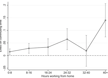
Finally, we investigate whether there are nonlinearities in the effect of hours working from home on commuting time. We do this by estimating a dummy specification, in which the variable denoting weekly hours spent working from home is divided up into 7 categories (0, 0–8, 8–16, 16–24, 42–32, 32–40, and 40+). The model, presented in the column (1) of Table9in “Appendix A”, is an alternative version of Table 5

column (3), and the marginal effects of the dummies are depicted in Fig.4. While the graph does not show significant effects of telecommuting categories 16–24 and 32–40, the overall pattern of point estimates follows a somewhat linear pattern, at least up until the 24–32 h mark. Considering the observed pattern, and the significance of the other dummies, we may conclude that the parametric approach in Table5column (3) is a reasonable approximation of the nonparametrically estimated shape of the relationship, and as it is more efficient it has our preference. In Table 9 columns (2–4) we show the results of this dummy specification using the other identification strategies, and in all specifications the pattern is roughly linear until 24–32 h.

In conclusion, the main result—that the effect of telecommuting on commuting time remains positive after controlling for sorting—is robust to identification based on the timing and intensity of telecommuting, and to an identification strategy based on a lagged dependent variable. A “long-difference” model suggests our estimates are somewhat conservative, and a linear specification of average weekly hours working from home is not problematic.

5 Conclusion

-.05

0

.05

.1

.15

.2

Effect on commuting time

0-8 8-16 16-24 24-32 32-40 40+ Hours working from home

Fig. 4Nonlinear effect of hours working from home. No telecommuting is the reference category. The dots represent the point estimates, the vertical lines represent the 95% confidence intervals, and the dashed horizontal line represents zero

that should be accounted for. On the one hand, the effects of commuting time on labour search and labour mobility suggest that telecommuters have a higher value of one-way commuting time, despite their lower commuting frequency, which would lead to a downward bias in OLS estimates of the effect of telecommuting on commuting time. However, using fixed effects to control for (stationary) preferences of individuals, our analysis shows that OLS estimates are biased upward in the range of 50–128%. This suggests that both residential- and commuting preferences distort OLS findings, and that the bias due to residential sorting is stronger.

Our preferred estimates suggest that moving from a situation with no telecommut-ing, telecommuting allows people to accept 5% longer commuting times on average, and every additional 8 weekly hours of working from home are associated with 3.5% longer commuting times. The main result of this study is that the effect of telecommut-ing on commuttelecommut-ing time remains positive and significant, after controlltelecommut-ing for individual preferences. This result is robust to a number of sensitivity checks in which we apply alternative identification methods, and allow for a nonlinear effect of weekly hours working from home.

changesin telecommuting, unrelated to changes in commuting time to assess the one-way causal effect. Finally, our fixed effects model corrects for the bias induced by preference-based sorting only to the extent that these preferences aretime-invariant. We are hopeful that our extensive list of control variables captures remaining changes in these preferences, and we note that including fixed effects may at least capture more of the sorting bias than OLS models.

In line with earlier work, our results suggest that the travel savings made by working one or several days at home are not fully offset by the positive effects on commut-ing distance alone (Jiang2008; Andreev et al.2010; Zhu 2012). Beyond that, this paper stresses the effects of telecommuting on the geographical territory of labour markets. Next to reducing the labour accessibility gap between central and remote areas, telecommuting may also allow the externalities associated with the size of local labour markets, including improved searching and matching and less unfilled vacan-cies (Moretti2011), to be increasingly generated across greater geographical areas, and through wider infrastructure networks (Burger and Meijers2016). Further research may focus on the welfare effects associated with a wider geographical extent of labour markets.

Acknowledgements Funding was provided by Nederlandse Organisatie voor Wetenschappelijk Onderzoek (NL) (Grant No. 452-14-004).

Open Access This article is distributed under the terms of the Creative Commons Attribution 4.0 Interna-tional License (http://creativecommons.org/licenses/by/4.0/), which permits unrestricted use, distribution, and reproduction in any medium, provided you give appropriate credit to the original author(s) and the source, provide a link to the Creative Commons license, and indicate if changes were made.

Appendix A

This appendix contains tables with regression results from the sensitivity analysis. Table6presents models based on a sample that only consists of telecommuters. Table7

shows the lagged dependent variable models. Table8shows the “long differences” models, and Table9shows models in which we allow for a nonlinear specification of weekly telecommuting hours.

Table 6Sensitivity regressions I: telecommuting sample

(1) (2) (3)

Telecommuting 0.0453*** (0.0148)

Telecommuting 1 day/month 0.0590***

(0.0197) Telecommuting 2 days/month 0.0482**

Table 6continued

(1) (2) (3)

Telecommuting 3 days/month 0.0311

(0.0197)

Telecommuting > 3 days/month 0.0125 (0.0199)

Telecommuting weekly hours 0.00407***

(0.000868)

Indiv. fixed effects Yes Yes Yes

Year dummies Yes Yes Yes

Control variables Yes Yes Yes

Observations 8309 8309 8309

R-squared 0.773 0.773 0.773

Robust std. errors in parentheses. In columns (1–2) no telecommuting is the reference category. Control variables are the same as in Tables4and5

***p< 0.01; **p< 0.05; *p< 0.1

Table 7Sensitivity regressions II: lagged dependent variable

(1) (2) (3)

Telecommuting 0.0526***

(0.0128)

Telecommuting 1 day/month 0.0334*

(0.0180)

Telecommuting 2 days/month 0.0783*** (0.0180)

Telecommuting 3 days/month 0.0411**

(0.0165) Telecommuting > 3 days/month 0.0268

(0.0197)

Telecommuting weekly hours 0.00398*** (0.00101)

Commuting time att−1 (log) 0.726*** 0.726*** 0.725***

(0.0101) (0.0101) (0.0102)

Indiv. fixed effects Yes Yes Yes

Year dummies Yes Yes Yes

Control variables Yes Yes Yes

Observations 11,090 11,090 11,090

R-squared 0.617 0.618 0.618

Robust std. errors in parentheses. In columns (1–2) and (4) no telecommuting is the reference category. Control variables are the same as in Tables4and5

Table 8Sensitivity regressions III: long differences

(1) (2) (3)

Telecommuting 0.277***

(0.0777)

Telecommuting 1 day/month 0.224** (0.0911)

Telecommuting 2 days/month 0.187

(0.121) Telecommuting 3 days/month 0.234*

(0.132)

Telecommuting > 3 days/month 0.0442 (0.0987)

Telecommuting weekly hours 0.0233***

(0.00416)

Indiv. fixed effects Yes Yes Yes

Year dummies Yes Yes Yes

Control variables Yes Yes Yes

Observations 1032 1032 1032

R-squared 0.759 0.756 0.767

Robust std. errors in parentheses. In columns (1–2) no telecommuting is the reference category. Control variables are the same as in Tables4and5

***p< 0.01; **p< 0.05; *p< 0.1

Table 9Sensitivity regressions IV: nonlinear telecommuting hours

(1) (2) (3) (4)

Telecommuting weekly hours 0–8 0.0348*** 0.0349** 0.0375** 0.115 (0.0133) (0.0150) (0.0176) (0.0743)

Telecommuting weekly hours 8–16 0.0659*** 0.0609** 0.0841*** 0.317***

(0.0230) (0.0260) (0.0310) (0.119) Telecommuting weekly hours 16–24 0.0767* 0.0696 0.0773 0.627***

(0.0393) (0.0426) (0.0534) (0.225)

Telecommuting weekly hours 24–32 0.149*** 0.142*** 0.159*** 0.685* (0.0491) (0.0518) (0.0502) (0.386)

Telecommuting weekly hours 32–40 0.0431 0.0409 0.123 1.024**

(0.0722) (0.119) (0.0784) (0.438) Telecommuting weekly hours 40+ 0.323*** 0.319*** 0.0526 1.812***

(0.0778) (0.104) (0.115) (0.493)

Commuting time att−1 (log) 0.101***

Table 9continued

(1) (2) (3) (4)

Model FE TC sample LDV LD

Indiv. fixed effects Yes Yes No Yes

Year dummies Yes Yes Yes Yes

Control variables Yes Yes Yes Yes

Observations 15,505 8309 6110 1032

R-squared 0.797 0.773 0.850 0.766

Robust std. errors in parentheses. No telecommuting is the reference category. Control variables are the same as in Tables4and5

FEfixed effects,TCtelecommuting,LDVlagged dependent variable,LDlong differences ***p< 0.01; **p< 0.05; *p< 0.1

References

Alonso W (1974) Location and land use: toward a general theory of land rent. Harvard University Press, Cambridge

Andreev P, Salomon I, Pliskin N (2010) Review: state of teleactivities. Transp Res C Emerg Technol 18(1):3–20.https://doi.org/10.1016/j.trc.2009.04.017

Angrist J, Pischke J (2008) Mostly harmless econometrics: an empiricist’s companion. Princeton University Press, Princeton

Bernardino A (2017) Telecommuting: modelling the employer’s and the employee’s decision-making pro-cess. Routledge, London

Büchel F, Van Ham M (2003) Overeducation, regional labor markets, and spatial flexibility. J Urban Econ 53(3):482–493.https://doi.org/10.1016/S0094-1190(03)00008-1

Burger MJ, Meijers EJ (2016) Agglomerations and the rise of urban network externalities. Pap Reg Sci 95(1):5–15.https://doi.org/10.1111/pirs.12223

Burger MJ, Meijers EJ, Van Oort FG (2014) Multiple perspectives on functional coherence: heterogeneity and multiplexity in the randstad. Tijdschr Econ Soc Geogr 105(4):444–464.https://doi.org/10.1111/t esg.12061

Cairncross F (1997) The death of distance: how the communication revolution is changing our lives. Harvard Business School Press, Boston

De Graaff T (2004) On the substitution and complementarity between telework and travel: a review and application. Research memorandum 16-2004, Vrije Universiteit Amsterdam.http://degree.ubvu.vu.n l/repec/vua/wpaper/pdf/20040016.pdf

Glaeser EL, Kahn ME (2004) Sprawl and urban growth. In: Henderson JV, Thisse JF (eds) Handbook of regional and urban economics, vol 4. Elsevier, Amsterdam, pp 2481–2527.https://doi.org/10.1016/s 1574-0080(04)80013-0

Gronberg T, Reed W (1994) Estimating workers’ marginal willingness to pay for job attributes using duration data. J Hum Resour 29(3):911–931.https://doi.org/10.2307/146258

Groot SPT, de Groot HLF, Smit MJ (2014) Regional wage differences in the Netherlands: micro evidence on agglomeration externalities. J Reg Sci 54(3):503–523.https://doi.org/10.1111/jors.12070

Gubins S, Verhoef ET (2014) Dynamic bottleneck congestion and residential land use in the monocentric city. J Urban Econ 80:51–61.https://doi.org/10.1016/j.jue.2013.09.001

Isacsson G, Karlström A, Swärdh JE (2013) The value of commuting time in an empirical on-the-job search model an application based on moments from two samples. Appl Econ 45(19):2827–2837.https://do i.org/10.1080/00036846.2012.678981

Kim SN, Mokhtarian PL, Ahn KH (2012) The Seoul of Alonso: new perspectives on telecommuting and residential location from South Korea. Urban Geogr 33(8):1163–1191. https://doi.org/10.2747/0272-3638.33.8.1163

Kim SN, Choo S, Mokhtarian PL (2015) Home-based telecommuting and intra-household interactions in work and non-work travel: a seemingly unrelated censored regression approach. Transp Res A Policy Pract 80:197–214.https://doi.org/10.1016/j.tra.2015.07.018

Kolko J (2012) Broadband and local growth. J Urban Econ 71(1):100–113.https://doi.org/10.1016/j.jue.2 011.07.004

Lund JR, Mokhtarian PL (1994) Telecommuting and residential location: theory and implications for com-mute travel in monocentric metropolis. Transportation research record 1463, pp 10–14.http://online pubs.trb.org/Onlinepubs/trr/1994/1463/1463-002.pdf

Mokhtarian PL, Salomon I, Choo S (2005) Measuring the measurable: why can’t we agree on the number of telecommuters in the U.S.? Qual Quant 39(4):423–452. https://doi.org/10.1007/s11135-004-6790-z

Moretti E (2011) Local labor markets. In: Ashenfelter OC, Card D (eds) Handbook of labor economics, vol 4. Elsevier, Amsterdam, pp 1237–1313.https://doi.org/10.1016/s0169-7218(11)02412-9

Muhammad S, Ottens HF, Ettema D, Jong T (2007) Telecommuting and residential locational preferences: A case study of the Netherlands. J Hous Built Environ 22(4):339–358.https://doi.org/10.1007/s1090 1-007-9088-3

Muhammad S, de Jong T, Ottens HFL (2008) Job accessibility under the influence of information and communication technologies, in the Netherlands. J Transp Geogr 16(3):203–216.https://doi.org/10.1 016/j.jtrangeo.2007.05.005

Muth RF (1969) Cities and housing. University of Chicago Press, Chicago Naisbitt J (1994) The global paradox. William Morrow & Co., New York

Nilles JM (1991) Telecommuting and urban sprawl: mitigator or inciter? Transportation 18(4):411–432.

https://doi.org/10.1007/BF00186567

Rhee HJ (2008) Home-based telecommuting and commuting behavior. J Urban Econ 63(1):198–216.https:// doi.org/10.1016/j.jue.2007.01.007

Salomon I (1985) Telecommunications and travel: substitution or modified mobility? J Transp Econ Policy.

https://doi.org/10.1080/09595238100185051

SCP (2016) Arbeidsaanbodpanel 1985 t/m 2014.https://doi.org/10.17026/dans-x8q-46p7

Toffler A (1980) The third wave. Bantam Books, New York

Van Ham M (2002) Job access, workplace mobility, and occupational achievement. Eburon, Delft Van Ommeren J (1998) A test for randomly sampling using duration observations. Appl Econ Lett

5(4):243–246.https://doi.org/10.1080/135048598354906

Van Ommeren J, Fosgerau M (2009) Workers’ marginal costs of commuting. J Urban Econ 65(1):38–47.

https://doi.org/10.1016/j.jue.2008.08.001

Van Ommeren J, Van Den Berg GJ, Gorter C (2000) Estimating the marginal willingness to pay for com-muting. J Reg Sci 40(3):541–563.https://doi.org/10.1111/0022-4146.00187

Van Wee B, Geurs KT, Chorus C (2013) Information, communication, travel behavior and accessibility. J Transp Land Use 6(3):1–16.https://doi.org/10.5198/jtlu.v6i3.282

Vermeulen W, Rouwendal J (2007) Housing supply and land use regulation in the Netherlands. SSRN Electr J.https://doi.org/10.2139/ssrn.1003955

Webber MM (1963) The post-city age. Daedalus 97(4):1091–1110.http://www.jstor.org/stable/20013413