Two Step Hybrid Block Method for Solving Nonlinear Jerk Equations

(1)

http://www.scirp.org/journal/jamp ISSN Online: 2327-4379

ISSN Print: 2327-4352

DOI: 10.4236/jamp.2019.78130 Aug. 26, 2019 1893 Journal of Applied Mathematics and Physics

Two-Step Hybrid Block Method for

Solving Nonlinear Jerk Equations

Bothayna S. H. Kashkari1, Sadeem Alqarni2,3

1_{Department of Mathematics, Faculty of Science, University of Jeddah, Jeddah, KSA} 2_{Department of Mathematics, Faculty of Science, King Abdulaziz University, Jeddah, KSA} 3_{Department of Mathematics, Faculty of Science, Al-Baha University, Al-Baha, KSA}

Abstract

In this paper, a block method with one hybrid point for solving Jerk equa-tions is presented. The hybrid point is chosen to optimize the local truncation errors of the main formulas for the solution and the derivative at the end of the block. Analysis of the method is discussed, and some numerical examples show that the proposed method is efficient and accurate.

Keywords

Nonlinear Jerk Equations, Hybrid Block Method, Zero Stable, Consistent, Convergent

1. Introduction

Jerk is the rate of acceleration change in physics; that is, the time derivative of acceleration, and as such the second velocity derivative, or the third time posi-tion derivative. The jerk is important in several mechanics and acoustics applica-tions. The Jerk vector is here resolved into tangential-normal and radial-transverse components for planar motion, and the normal component is expressed as an affine differential invariant recognized as the aberrancy. Several geometric properties of the Jerk vector are established for plane motion using known aber-rancy properties of curves [1].

Nonlinear third-order differential equations, known as nonlinear Jerk equa-tions, involving the third temporal displacement derivative, are of great interest in analyzing some structures which exhibit rotating and translating movements, such as robots or machine tools, where excessive Jerk leads to accelerated wear of transmissions and bearing elements, noisy operations and large contouring errors in discontinuities (such as corners) in the machining path [2].

How to cite this paper: Kashkari, B.S.H. and Alqarni, S. (2019) Two-Step Hybrid Block Method for Solving Nonlinear Jerk Equations. Journal of Applied Mathematics and Physics, 7, 1893-1910.

https://doi.org/10.4236/jamp.2019.78130

Received: July 24, 2019 Accepted: August 23, 2019 Published: August 26, 2019

http://creativecommons.org/licenses/by/4.0/

(2)

0 =0. The most general

function of Jerk, which is invariant in time-reversal and space-reversal and only nonlinear cubic, can be written as

2 2 3

0,

y′′′+αyy y′ ′′+βy y′ ′′ +δy y′+y′ +γy′= (2)

where the parameters are α β δ, , , and γ is constants. The current work is

motivated by optimizing local truncation errors in order to find a hybrid point in a two-step block method to have the most accurate solution for Jerk Equation (1). We organize this paper as follows: The next section illustrates the method derivation, Section 3 presents the analysis of the method involving order four, Section 4 presents the numerical examples showing the productivity of the new technique when it is contrasted with the different strategies proposed in the scientific writing.

2. Methodology

To derive two steps hybrid block method with one off-step point we have a po-lynomial of degree 6 as follows:

( )

6

0

,

j j j

y x p x a x

=

∑

 (3) with third derivative given by

( )

6

(

)(

)

3

1 2 j j .

j

y x p x j j j a x−

=

′′′  ′′′ =

∑

− − (4)

Substituting Equation (4) into Equation (3) gives

(

)

6

(

)(

)

3

, , , 1 2 j j .

j

f x y y y j j j a x −

=

′ ′′ =

∑

− − ₍₅₎

By interpolating Equation (3) at x_m+_j,j=0, ,1r and collocating Equation (5)

at xm+j,j=0, ,1, 2r we get a system of equations written in the matrix form

2 3 4 5 6

0

2 3 4 5 6

1

2 3 4 5 6

2

1 1 1 1 1 1

2 3

1 1 1

2 3

2 2 2

1 1 1

0 0 0 6 24 60 120

m m m m m m m r m r m r m r m r m r m m m m m m

m m m m r m r m r m m m m m m

a

x x x x x x

a

x x x x x x

a

x x x x x x

x x x

+ + + + + +

+ + +

 

 

 

1

3

4

5 1

6 2

m m r m

m m r m m

y y y

a f

+

   

   

=

   

   

(3)

DOI: 10.4236/jamp.2019.78130 1895 Journal of Applied Mathematics and Physics Solving the above system (by using Gaussian elimination method for solving the system of linear equations [8]) gives us the coefficients of the polynomial

, 0,1, , 6

j

a j=  .

By making the substitution x=xm+th, the polynomial in Equation (3) may

be written in the form:

(

)

3

1 ,

1

t r t r

α = −

−

(

)

(

)

3

4 3 2 3 2

0

4 3 2

1 8 22 2 13

240

27 5 5 5 5 ,

h

t t r r r rt rt

r

rt r t t t t

β = − − − + − +

− − + − + +

(

)

(

)

(

)

3

4 3 2 4 3 2

2 1 5 5 5 5 5 5 ,

120 3 2

r

h

t t r r r r t t t t

r r r

β = − − − + + − + − −

− +

(

) (

(

)

(

)

3

4 3 2 3 2

1

4 3 2

1 5 5 2 8

120 1

8 3 3 3 3 ,

h

t t r r r rt rt

r

rt r t t t t

β = − − − + + + −

−

− − − + + +

(

) (

(

)

(

)

3

4 3 2 3 2

2

4 3 2

1 2 2 2 3

240 2

3 .

h

t t r r r rt rt

r

rt r t t t t

β = − − + + + −

−

− − − + + +

(7)

Now, by evaluating the solution approximation at the point xm+2:

(

)

(

)

(

)

(

)

(

)

2 1

3 4 3 2 3 2

3 3 2 3 3

1 2

2 2 2 4

1 1

8 22 23 6 2 3

120 60

4 9 26 2 1

.

60 120

m m m r m

m m r

m m

r r

y y y y

r r r r

h r r r r h r r

f f

r r

h r r r h r r

f f + + + + + + − − = − + + − − − + − + − + + − + − + + − − + + − + (8)

Assess the approximation at the point of first derivative xm+2:

(

)

(

)

(

)

2 1

3 4 3 2

2

3 3 4

1 1

3 24 66 67 12

240

5 5 5 4

(40 ( 3 2))

m m m r m

m

m r

r r

hy y y y

r r r r

h r r r r

f r

h r r r r

f

r r r

(4)

DOI: 10.4236/jamp.2019.78130 1896 Journal of Applied Mathematics and Physics

(

)

(

)

(

)

(

)

3 4 3 2

1

3 4 3 2

2

3 15 15 137 116

120 1

2 2 3 12

.

80 2

m

h r r r r

f r

h r r r r

f r + + − + + − + − − − + + + − + − (9)

Evaluate the second derivative approximation at the point xm+2:

(

)

(

)

(

)

(

)

(

)

(

)

(

)

2 2 1

3 4 3 2

2

3 4 3 2

1

3 4 3 2

2

2 2 2

1 1

8 22 18 5

120

5 5 5 5

(60 ( 3 2))

5 5 75 77

60 1

2 2 42 81

.

120 2

m m m r m

m

m r

m

h y y y y

r r r r

h r r r r

f r

h r r r r

f

r r r

h r r r r

f r

h r r r r

f r + + + + + + ′′ = + − − − − + − + + + − + + + − − + − + + − + − − − + + + − + − (10)

We choose to optimize the local truncation errors in the Equation (8), Equa-tion (9) and EquaEqua-tion (10) to determine appropriate values for r EquaEqua-tion (8), Equation (9) and Equation (10). This choice at the end of the block ym+2, ym′+2

and ym′′+2, which result respectively in

(

)

(

)

( )

_{( )}

(

)

( )

_{( )}

(

)

2 7 7

5 4 3 2

8 8

6 5 4 3 2

;

3 18 24 24 53 10

10080

9 33 47 205 51 327 42 , 100800

m m

m

y x h

h y x

r r r r r

h y x

r r r r r r

+ = − − + + − + − − − + + − + 

(

)

(

)

( )

₍

₎

( )

_{( )}

(

)

2 7 (7)

5 4 3 2

8 8

6 5 4 3 2

;

9 54 72 72 117 44

20160

27 99 141 615 237 729 556 ,

201600

m

y x h

h y x

r r r r r

h y x

r r r r r r

+ ′ = − + − − + + + − + + − − + + 

(

)

(

)

( )

_{( )}

(

)

( )

_{( )}

(

)

2 7 7

5 4 3 2

8 8

6 5 4 3 2

;

6 8 8 8 41

3360

9 33 47 205 205 135 1195 . 100800

m m

m

y x h

h y x

r r r r r

h y x

r r r r r r

+ ′′ = − − + + + − − − − + + + −  (11)

Determine the r values equating to zero the 7

h coefficients in the local trun-cation error formulas in Equation (11), and we obtain the system

5 4 3 2

3r 18r 24r 24r 53r 10 0,

− + − − + − =

5 4 3 2

9r 54r 72r 72r 117r 44 0,

(5)

5 4 3 2

6 8 8 8 41 0.

r r r r r

7 ( )7

( )

8 26 ; 84685 m h y

y′′ x h ≈− +O h



To obtain a two-step hybrid block solution method for solving Equation (1), we evaluate p x′

( )

,p′′

( )

x at the points xm,xm r+ ,xm+₁, we get the following

block of six equations

(

)

(

)

(

)

(

)

(

)

(

)

(

)

(

)

1

3 3 2

2

3 3 2

1

3 3 2

2

1 1

8 22 5

240

5 5 5

120 3 2

5 5 3

120 1

2 2 1

, 240 2

m m m r m

m

m r

m

r r

hy y y y

r r r r

h r r r

f

h r r r

f

r r

h r r r r

f r

h r r r r

f r + + + + + + ′ = − − + − − − + − + − + + + − + − + + − + − − + + − − −

(

)

(

)

(

)

(

)

(

)

(

)

(

)

(

)

2 1

3 4 3 2

2

3 4 3 2

1

3 4 3 2

2

2 2 2

1 1

8 22 28 10

120

5 5 5 10

60 3 2

5 5 35 22

60 1

2 2 8 4

, 120 2

m m m r m

m

m r

m

h y y y y

r r r r

h r r r r

f r

h r r r r

f

r r r

h r r r r

f r

h r r r r

f r + + + + + ′′ = + − − − − + − + − − + + − − − + − + + − + − − − + + − + + −

(

)

(

)

1

3 4 3 2

1 2 1

1 1

2 13 28 22 5

240

m r m m r m

m

r r r

hy y y y

r r r r

h r r r r

(6)

(

)

(

)

(

)

(

)

(

)

3 3 2

1

3 4 3 2

2

4 15 10 5

120 2

2 7 2 3

120

2 5 2 2 1

, 240 2

m r

m

h r r r

f r

h r r r r

f

h r r r r r

f r + + + − + + + − − + + − + − + + − + −

(

)

(

)

(

)

(

)

(

)

(

)

(

)

(

)

2 1

3 4 3 2

2

3 4 3 2

1

3 4 3 2

2

2 2 2

1 1

4 22 38 22 5

120

14 55 55 5 5

60 3 2

4 15 5 5 3

60 1

4 8 2 2 1

, 120 2

m r m m r m

m

m r

m

h y y y y

r r r r

h r r r r

f r

h r r r r

f

r r r

h r r r r

f r

h r r r r

f r + + + + + + ′′ = + − − − − + − + + − + − + + − − + − + + − − − − + + − + −

(

)

(

)

(

)

(

)

(

)

1 1

3 4 3 2

3 2

3 3 2

1

3 3

2

1 1 2

1 1

8 22 21 6

240 2 3

120

4 9 8

120 2 1

, 240

m m m r m

m

m r

m

r r

hy y y y

r r r r

h r r r r

f r

h r r

f r

h r r r

f

h r r

f + + + + + + − − ′ = − + + − − − + − + − − + + + − + + − − − + −

(

)

(

)

(

)

(

)

(

)

(

)

(

)

2 1 1

3 4 3 2

2

3 4 3 2

1

3 4 3 2

2

2 2 2

1 1

8 22 28 10

120

5 5 5 10

60 ( 3 2)

5 5 35 22

60 1

2 2 8 4

.

120 2

m m m r m

m

m r

m

h y y y y

r r r r

h r r r r

f r

h r r r r

f

r r r

h r r r r

f r

h r r r r

f r + + + + + + ′′ = + − − − − + − + − − + + − − − + − + + − + − − − + + − + + − (13)

3. Characteristics of the Method

(7)

DOI: 10.4236/jamp.2019.78130 1899 Journal of Applied Mathematics and Physics to establish their validity.

3.1. Order of the Method

is a sufficiently differentiable function, the linear difference operator

 associated with the implicit two-step block hybrid method is considered in Equation (8), Equation (9), Equation (10), Equation (13), that is given

( )

(

)

(

)

(

)

(

)

2 3

;

m j m j m

j

j m j m

z x h z x jh h z x jh

h z x jh h z x jh

κ τ

γ ξ

′

  = + − +

 

′′ ′′′

− + − +

∑



(15)

0, ,1, 2

j= r where the κ τ γ_j, _j, _j and ξ_j are respectively the vector

col-umns of the matrices A B C, , and V.

Expanding z x

(

m+jh

) (

,z x′ m+ jh

) (

,z′′ xm+ jh

)

and z′′′

(

xm+jh

)

in Taylor series about xm we get

( )

2

( )

_{( )}

0 1 2

; q q

m m m m q m

z x h C y x C hy x′ C h y′′ x C h y x

  = + + + + +

   

 (16)

with C0=C1=C2==C6=0 and

(

6 20

7

4 4

3 5

4 3

9.437739543552612 10 , 9.617040306545119 10 ,

3.070200924962517 10 , 4.913128762599697 10 ,

2.144715335032775 10 ,8.823816935161847 10 ,

4.504524331158401 10 , 3.184040914146728 10 ,

1.14181

C − −

− −

= × − ×

− × − ×

× ×

− × ×

− ₂

)

T

3120360736 10× −

Note that the proposed method has order p=4 at least [9].

3.2. Zero Stability

We can write the method as a vector As h→0 in Equation (14), we can write

the method as a vector form.

0 m 1 m 1 0

A Y −A Y − = where

(

)

T

(

)

T

2, 1, , 1 , 1, 1

m m m m r m m m m r

Y = y ₊ y ₊ y ₊ Y ₋ = y y ₋ y _{+ −}

0

1 0.6017954608298602 1.471021404061736

0 1 0

0 0 1

A

−

 

 

=  

 

(8)

DOI: 10.4236/jamp.2019.78130 1900 Journal of Applied Mathematics and Physics 1

0.1307740567681242 0 0

1 0 0

A

 

 

=  

 

 

The first characteristic polynomial

( )

[

] (

)

2

0 1

det 1 0

z A z A z z

ρ = − = − = _{, the roots of polynomials are}

1 2 0; 3 1

z =z = z = . Hence the block method is zero -stable [9].

3.3. Consistency

The block method has order p=4, in case p≥1, this is a sufficient condition

to be consistent with the associated block method [10].

3.4. Convergence

We can establish the convergence of the two-step with three points hybrid block method if and only if it is consistent and zero stable [11].

3.5. Region of Absolute Stability

As we mentioned earlier, zero-stability is a concept of the numerical method behavior for h→0. To decide whether a numerical method will produce good

results with a given value of h>0, we need a concept of stability that is

differ-ent from zero-stability. In most numerical methods intended to solve problems of third order, the stability properties are usually analyzed by considering the li-near equation given by the Dalquist test [11].

( )

3

y′′′ = −λ y x (17)

This problem has bounded solutions for λ ≥0 that tend to zero for x→ ∞.

We will define the region where the numerical method reproduces the manner of the exact solutions. Let us explain the procedure for obtaining such a region. Our method has nine equations in which there are four different terms of first derivatives: ym′,ym r′+ ,ym′+1,ym′+2, and second derivative: ym′′ ′′,ym r+ ,y′′m+1,ym′′+2 and

one intermediate values ym r+ . Let us depict the procedure to gain such a region

[12], We eliminated these terms from the equations system by using mathematica, and get a recurrence equation in the terms ym,ym+1,ym+2. This

1.433653893592262 10 5.520254762660736 10

3.674797669760869 10

P z z

z

= − × + ×

+ ×

( )

109 108 3

107 6

5.734615574369057 10 8.898486741828162 10

3.679066781172749 10

Q z z

z

= × − ×

+ ×

( )

109 109

108 3 107 4

106 6

4.300961680776793 10 2.867307787184524 10

1.211231358386333 10 6.261663213347228 10

4.300976789540145 10

S z z

z z

z

= − × + ×

− × − ×

+ ×

(9)

DOI: 10.4236/jamp.2019.78130 1901 Journal of Applied Mathematics and Physics Through its characteristic equation, we study the extent boundedness of their solutions to define the region of stability. The root causes of the characteristic equation

(

) (

)

109 107 3

106 6 2 109

108 3 107 6

109

1.433653893592262 10 5.520254762660736 10

3.674797669760869 10 5.734615574369057 10

8.898486741828162 10 3.679066781172749 10

4.300961680776793 10 2.867307787184524 1

z

z x

z z x

− × + ×

+ × + ×

− × + ×

+ −

(

× + ×

)

109

108 3 107 4

106 6

0

1.211231358386333 10 6.261663213347228 10

4.300976789540145 10 0

z

z z

z

− × − ×

+ × =

(20)

are

1 6 3

12 10

9

2

4509981306728599 67748616455391176 1759485240133103872

( (121468655749357324985383025377280 86645450698059554742358457188352

6085569311397395324399777440858112 266604101119524264596197

x

z z

z

= −

+ −

× +

− − 7

6 4

3

1549077504

125054287321797496835881016603181056 93404454773980569973608059370471424

936741366582786806117795003533099008 1547894155123122963374310449590829056 77394707756156767979316399120475

z

z z

+ −

− +

+

3 6

7504)

546043788941838592z 22576103367311352z 3518970480266213376)

− + +

2 6 3

12 10

9

2

4509981306728599 67748616455391176 1759485240133103872

( (121468655749357324985383025377280 86645450698059554742358457188352

6085569311397395324399777440858112 2666041011195242645961971

x

z z

z

=

+ −

× +

− − 7

6 4

3

549077504

125054287321797496835881016603181056 93404454773980569973608059370471424

936741366582786806117795003533099008 1547894155123122963374310449590829056 773947077561567679793163991204757

z

z z

+ −

− +

+

3 6

504)

546043788941838592z 22576103367311352z 3518970480266213376)

+ − −

The roots of the characteristic equation must be less than 1, for the method to be stable. The stability region for the method has shown in Figure 1.

4. Numerical Examples

Example 1: Consider the Jerk equation in the following form:

y′′′= − +y′ yy y′ ′′ (21)

With initial conditions: y

( )

0 =0,y′

( )

0 =B y, ′′

( )

0 =0, and exact solution:

( )

(

2 2

)

( )

2

(

)

3

sin 9 48 48 sin sin 3

96

B B

y x = Ω +x − B − + Ω Ω −x B Ωx

Ω Ω

where 1 2

4 2 B

Ω = + .

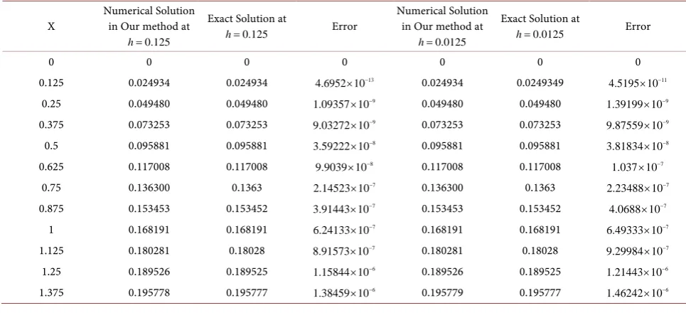
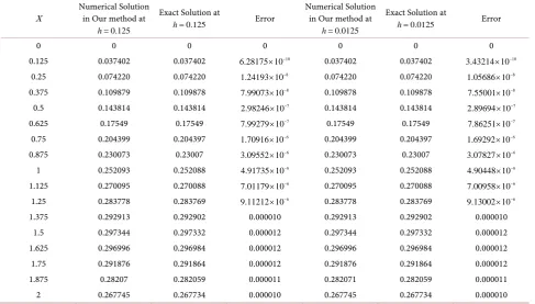
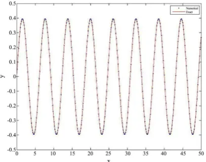
Tables 1-3 show the absolute Errors at h=0.125, 0.0125 and 0.2, 0.3, 0.4

(10)

be-DOI: 10.4236/jamp.2019.78130 1902 Journal of Applied Mathematics and Physics tween our method and result in [13] is proposed in Table 4 and Table 5. It is seen in Figures 2-4 the method gives a good approximation in the interval

[

0, 50

]

x∈ and B=0.2, 0.3, 0.4 respectively.

Example 2: Consider the Jerk equation in the following form: 2

y′′′= − −y′ y y′ ′′ (22)

With initial conditions: y

( )

0 =0,y′

( )

0 =B y, ′′

( )

0 =0, and exact solution:

( )

(

)

( )

(

)

( )

(

)

2 2 2

3

3 2 3 2 2

sin 9 48 48 sin

96

12 48 48 cos sin 3

B B

y x x B x

B x x B x

= Ω + − Ω − + Ω Ω

Ω Ω

+ Ω + Ω − Ω Ω − Ω Ω

where 2

1 2

4 B

Ω =

[image:10.595.203.518.46.718.2]

− .

[image:10.595.263.488.520.703.2]

Figure 1. Region of absolute stability.

(11)

[image:11.595.261.486.67.248.2] [image:11.595.261.488.282.460.2]

DOI: 10.4236/jamp.2019.78130 1903 Journal of Applied Mathematics and Physics Figure 3. The solution of Example 1 at h=0.125, B=0.3.

Figure 4. The solution of Example 1 at h=0.125, B=0.4.

Table 1. Absolute error of numerical solutions at B=0.2.

X Numerical Solution in Our method at

0.125

h=

Exact Solution at

0.125

h= Error

Numerical Solution in Our method at

0.0125

h=

Exact Solution at

0.0125

h= Error

0 0 0 0 0 0 0

0.125 0.024934 0.024934 13

4.6952 10× − 0.024934 0.0249349 11

4.5195 10× −

0.25 0.049480 0.049480 9

1.09357 10× − 0.049480 0.049480 9

1.39199 10× −

0.375 0.073253 0.073253 9

9.03272 10× − 0.073253 0.073253 9

9.87559 10× −

0.5 0.095881 0.095881 8

3.59222 10× − 0.095881 0.095881 8

3.81834 10× −

0.625 0.117008 0.117008 8

9.9039 10× − 0.117008 0.117008 7

1.037 10× −

0.75 0.136300 0.1363 7

2.14523 10× − 0.136300 0.1363 7

2.23488 10× −

0.875 0.153453 0.153452 7

3.91443 10× − 0.153453 0.153452 7

4.0688 10× −

1 0.168191 0.168191 7

6.24133 10× − 0.168191 0.168191 7

6.49333 10× −

1.125 0.180281 0.18028 7

8.91573 10× − 0.180281 0.18028 7

9.29984 10× −

1.25 0.189526 0.189525 6

1.15844 10× − 0.189526 0.189525 6

1.21443 10× −

1.375 0.195778 0.195777 6

1.38459 10× − 0.195779 0.195777 6

[image:11.595.55.538.512.732.2]

(12)

Continued

1.5 0.198937 0.198935 6

1.53404 10× − 0.198937 0.198935 6

1.63819 10× −

1.625 0.198949 0.198948 6

1.58573 10× − 0.198949 0.198948 6

1.72019 10× −

1.75 0.195816 0.195815 6

1.53899 10× − 0.195817 0.195815 6

1.70703 10× −

1.875 0.189589 0.189587 6

1.41336 10× − 0.189589 0.189587 6

1.61747 10× −

2 0.180367 0.180365 6

1.24351 10× − 0.180367 0.180365 6

[image:12.595.56.544.190.467.2]

1.48465 10× − Table 2. Absolute error of numerical solutions at B=0.3.

0.125

h=

Exact Solution at

0.125

h= Error

0.0125

h=

Exact Solution at

0.0125

h= Error

0 0 0 0 0 0 0

0.125 0.037402 0.037402 10

6.28175 10× − 0.037402 0.037402 10

3.43214 10× −

0.25 0.074220 0.074220 8

1.24193 10× − 0.074220 0.074220 8

1.05686 10× −

0.375 0.109879 0.109878 8

7.99073 10× − 0.109878 0.109878 8

7.55001 10× −

0.5 0.143814 0.143814 7

2.98246 10× − 0.143814 0.143814 7

2.89694 10× −

0.625 0.17549 0.17549 7

7.99279 10× − 0.17549 0.17549 7

7.86251 10× −

0.75 0.204399 0.204397 6

1.70916 10× − 0.204399 0.204397 6

1.69292 10× −

0.875 0.230073 0.23007 6

3.09552 10× − 0.230073 0.23007 6

3.07827 10× −

1 0.252093 0.252088 6

4.91735 10× − 0.252093 0.252088 6

4.90448 10× −

1.125 0.270095 0.270088 6

7.01179 10× − 0.270095 0.270088 6

7.00958 10× −

1.25 0.283778 0.283769 6

9.11212 10× − 0.283778 0.283769 6

9.13002 10× −

1.375 0.292913 0.292902 0.000010 0.292913 0.292902 0.000010

1.5 0.297344 0.297332 0.000012 0.297344 0.297332 0.000012

1.625 0.296996 0.296984 0.000012 0.296996 0.296984 0.000012

1.75 0.291876 0.291864 0.000012 0.291876 0.291864 0.000012

1.875 0.28207 0.282059 0.000011 0.282071 0.282059 0.000011

[image:12.595.55.542.502.731.2]

2 0.267745 0.267734 0.000010 0.267745 0.267734 0.000010

0.125

h=

Exact Solution at

0.125

h= Error

0.0125

h=

Exact Solution at

0.0125

h= Error

0 0 0 0 0 0 0

0.125 0.049869 0.049869 9

2.46607 10× − 0.049869 0.049869 9

1.4462 10× −

0.25 0.098960 0.098960 8

5.11558 10× − 0.098961 0.098961 8

4.45237 10× −

0.375 0.146501 0.146501 7

3.34007 10× − 0.146501 0.146501 7

3.17797 10× −

0.5 0.191739 0.191738 6

1.25262 10× − 0.191739 0.191738 6

1.21922 10× −

0.625 0.233947 0.233943 6

3.36066 10× − 0.233947 0.233943 6

3.30604 10× −

0.75 0.272436 0.272428 6

7.18675 10× − 0.272436 0.272428 6

7.10926 10× −

0.875 0.306566 0.306553 0.000013 0.306566 0.306553 0.000012

1 0.33576 0.335739 0.000021 0.33576 0.335739 0.000020

1.125 0.359513 0.359483 0.000029 0.359513 0.359483 0.000029

1.25 0.377408 0.37737 0.000038 0.377408 0.37737 0.000037

1.375 0.389127 0.389082 0.000045 0.389127 0.389082 0.000045

(13)

Continued

1.625 0.393308 0.393256 0.000052 0.393308 0.393256 0.000052

1.75 0.385695 0.385643 0.000051 0.385695 0.385643 0.000051

1.875 0.371756 0.371707 0.000048 0.371756 0.371707 0.000048

2 0.351742 0.351698 0.000044 0.351742 0.351698 0.000044

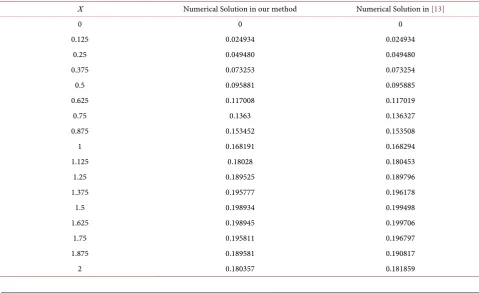
Table 4. Comparison between the numerical solution in our method and the method in [13], B=0.2,h=0.125.

X Numerical Solution in our method Numerical Solution in [13]

0 0 0

0.125 0.024934 0.024934

0.25 0.049480 0.049480

0.375 0.073253 0.073254

0.5 0.095881 0.095885

0.625 0.117008 0.117019

0.75 0.1363 0.136327

0.875 0.153453 0.153508

1 0.168191 0.168294

1.125 0.180281 0.180453

1.25 0.189526 0.189796

1.375 0.195778 0.196178

1.5 0.198937 0.199498

1.625 0.198949 0.199706

1.75 0.195816 0.196797

1.875 0.189589 0.190817

[image:13.595.62.539.176.435.2]

2 0.180367 0.181859

Table 5. Comparsion between the numerical solution in our method and the method in [13], B=0.4,h=0.125.

0 0 0

0.125 0.049869 0.049869

0.25 0.098960 0.098961

0.375 0.146501 0.146509

0.5 0.191739 0.191770

0.625 0.233947 0.234038

0.75 0.272436 0.272655

0.875 0.306566 0.307017

1 0.33576 0.336588

1.125 0.359513 0.360907

1.25 0.377408 0.379593

1.375 0.389127 0.392357

1.5 0.39446 0.398997

1.625 0.393308 0.399412

1.75 0.385695 0.393594

1.875 0.371756 0.381634

(14)

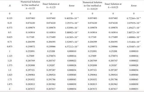
DOI: 10.4236/jamp.2019.78130 1906 Journal of Applied Mathematics and Physics Tables 6-8 show the absolute Errors at h=0.125, 0.0125 and

0.2, 0.3, 0.4

B= respectively. Example 2 was solved in [13], the comparison be-tween our method and result in [13] is proposed in Table 9 and Table 10. It is seen in Figures 5-7 the method gives a good approximation in the interval

[

0, 50

]

[image:14.595.274.476.346.507.2]

x∈ and B=0.2, 0.3, 0.4 respectively.

[image:14.595.273.477.540.700.2]

(15)

[image:15.595.57.541.89.390.2]

DOI: 10.4236/jamp.2019.78130 1907 Journal of Applied Mathematics and Physics Table 6. Absolute error of numerical solutions at B=0.2.

X

0.125

h=

Exact Solution at

0.125

h= Error

0.0125

h=

Exact Solution at

0.0125

h= Error

0 0 0 0 0 0 0

0.125 0.024934 0.024934 11

3.89579 10× − 0.024934 0.024934 11

8.68102 10× −

0.25 0.049480 0.049480 9

2.37202 10× − 0.049480 0.049480 9

2.68466 10× −

0.375 0.073253 0.073253 8

1.83415 10× − 0.073253 0.073253 8

1.92163 10× −

0.5 0.095881 0.095881 8

7.26168 10× − 0.095881 0.095881 8

7.49309 10× −

0.625 0.117008 0.117008 7

2.01662 10× − 0.117008 0.117008 7

2.06392 10× −

0.75 0.1363 0.1363 7

4.44143 10× − 0.1363 0.1363 7

4.53178 10× −

0.875 0.153452 0.153452 7

8.29786 10× − 0.153452 0.153452 7

8.45282 10× −

1 0.168191 0.16819 6

1.3665 10× − 0.168191 0.16819 6

1.39175 10× −

1.125 0.18028 0.180278 6

2.03637 10× − 0.18028 0.180278 6

2.07483 10× −

1.25 0.189525 0.189522 6

2.79641 10× − 0.189525 0.189522 6

2.85251 10× −

1.375 0.195777 0.195773 6

3.59097 10× − 0.195777 0.195773 6

3.66902 10× −

1.5 0.198934 0.198929 6

4.36561 10× − 0.198934 0.198929 6

4.47017 10× −

1.625 0.198945 0.19894 6

5.08301 10× − 0.198945 0.19894 6

5.21817 10× −

1.75 0.195811 0.195805 6

5.73169 10× − 0.195811 0.195805 6

5.90079 10× −

1.875 0.189581 0.189575 6

6.32606 10× − 0.189581 0.189575 6

6.53163 10× −

2 0.180357 0.18035 6

6.89847 10× − 0.180357 0.18035 6

7.14149 10× −

X

0.125

h=

Exact Solution at

0.125

h= Error

0.0125

h=

Exact Solution at

0.0125

h= Error

0 0 0 0 0 0 0

0.125 0.037402 0.037402 10

9.40558 10× − 0.037402 0.037402 10

6.72264 10× −

0.25 0.074220 0.074220 8

2.25371 10× − 0.074220 0.074220 8

2.07935 10× −

0.375 0.109879 0.109878 7

1.53599 10× − 0.109878 0.109878 7

1.49427 10× −

0.5 0.143814 0.143814 7

5.88902 10× − 0.143814 0.143814 7

5.80723 10× −

0.625 0.17549 0.175489 6

1.61265 10× − 0.17549 0.175489 6

1.60006 10× −

0.75 0.204399 0.204395 6

3.52997 10× − 0.204399 0.204395 6

3.51404 10× −

0.875 0.230072 0.230066 6

6.57212 10× − 0.230072 0.230066 6

6.55487 10× −

1 0.252091 0.25208 0.000010 0.252091 0.25208 0.000010

1.125 0.27009 0.270074 0.000016 0.27009 0.270074 0.000016

1.25 0.283769 0.283747 0.000022 0.283769 0.283747 0.000022

1.375 0.292898 0.29287 0.000028 0.292898 0.29287 0.000028

1.5 0.297321 0.297287 0.000034 0.297321 0.297287 0.000034

1.625 0.296964 0.296924 0.000040 0.296964 0.296924 0.000040

1.75 0.291832 0.291786 0.000045 0.291832 0.291786 0.000045

1.875 0.282012 0.281962 0.000050 0.282013 0.281962 0.000050

[image:15.595.59.538.421.730.2]

(16)

[image:16.595.57.537.445.738.2]

DOI: 10.4236/jamp.2019.78130 1908 Journal of Applied Mathematics and Physics Table 8. Absolute error of numerical solutions at B=0.4.

X

0.125

h=

Exact Solution at

0.125

h= Error

0.0125

h=

Exact Solution at

0.0125

h= Error

0 0 0 0 0 0 0

0.125 0.049869 0.049869 9

3.86139 10× − 0.049869 0.049869 9

2.91296 10× −

0.25 0.098960 0.098960 8

9.62982 10× − 0.098960 0.09896 8

9.01239 10× −

0.375 0.146501 0.146501 7

6.62938 10× − 0.146501 0.146501 7

6.47732 10× −

0.5 0.191739 0.191736 6

2.55096 10× − 0.191739 0.191736 6

2.51913 10× −

0.625 0.233946 0.233939 6

6.99674 10× − 0.233946 0.233939 6

6.9439 10× −

0.75 0.272434 0.272419 0.000015 0.272434 0.272419 0.000015

0.875 0.306562 0.306533 0.000028 0.306561 0.306533 0.000028

1 0.335749 0.335702 0.000046 0.335749 0.335702 0.000046

1.125 0.359492 0.359422 0.000069 0.359492 0.359422 0.000069

1.25 0.37737 0.377275 0.000095 0.37737 0.377275 0.000095

1.375 0.389065 0.388942 0.000122 0.389065 0.388942 0.000122

1.5 0.394363 0.394214 0.000149 0.394363 0.394214 0.000149

1.625 0.393169 0.392994 0.000174 0.393169 0.392994 0.000174

1.75 0.385503 0.385307 0.000196 0.385504 0.385307 0.000196

1.875 0.371507 0.371289 0.000217 0.371507 0.371289 0.000217

2 0.351432 0.351193 0.000238 0.351432 0.351193 0.000238

Table 9. Comparsion between the numerical solution in our method and the method in [13], B=0.2,h=0.125.

0 0 0

0.125 0.024934 0.024934

0.25 0.049480 0.049480

0.375 0.073253 0.073254

0.5 0.095881 0.095885

0.625 0.117008 0.117019

0.75 0.1363 0.136327

0.875 0.153452 0.153508

1 0.168191 0.168294

1.125 0.18028 0.180453

1.25 0.189525 0.189796

1.375 0.195777 0.196178

1.5 0.198934 0.199498

1.625 0.198945 0.199706

1.75 0.195811 0.196797

1.875 0.189581 0.190817

(17)

[image:17.595.59.542.87.395.2]

DOI: 10.4236/jamp.2019.78130 1909 Journal of Applied Mathematics and Physics Table 10. Comparison between the numerical solution in our method and the method in [13], B=0.4.

0 0 0

0.125 0.049869 0.049869

0.25 0.098960 0.098961

0.375 0.146501 0.146509

0.5 0.191739 0.191770

0.625 0.233946 0.234038

0.75 0.272434 0.272655

0.875 0.306562 0.307017

1 0.335749 0.336588

1.125 0.359492 0.360907

1.25 0.37737 0.379593

1.375 0.389065 0.392357

1.5 0.394363 0.398997

1.625 0.393169 0.399412

1.75 0.385503 0.393594

1.875 0.371507 0.381634

2 0.351432 0.363718

5. Conclusion

A two-step with one hybrid point was proposed and proceeded as a self-starting method for solving nonlinear Jerk equations. We considered one hybrid point and specified for approximation after optimizing local truncation errors re-lated to the main formula. Therefore, our method’s good convergent and sta-bility properties make it attractive for the numerical solution of nonlinear problems. The method presented is zero stable, consistent and convergence of four-algebraic order. The numerical results and figures show their efficiency and precision compared to other methods in the literature.

Conflicts of Interest

The authors declare no conflicts of interest regarding the publication of this paper.

References

[1] Schot, S.H. (1978) Jerk: The Time Rate of Change of Acceleration. American Jour-nal of Physics, 46, 1090-1094.https://doi.org/10.1119/1.11504

[2] Anu, N. and Marinca, V. (2016) Approximate Analytical Solutions to Jerk Equa-tions. Dynamical Systems: Theoretical and Experimental Analysis, Łódź, 7-10 De-cember 2015, 169-176.https://doi.org/10.1007/978-3-319-42408-8_14

(18)

Jerk Equations. Journal of Sound and Vibration, 271, 671-683.

https://doi.org/10.1016/S0022-460X(03)00299-2

[4] Momoniat, E. and Mahomed, F. (2010) Symmetry Reduction and Numerical Solu-tion of a Third-Order ODE from Thin Film Flow. Mathematical and Computational Applications, 15, 709-719.https://doi.org/10.3390/mca15040709

[5] Bhrawy, A. and Abd-Elhameed, W. (2011) New Algorithm for the Numerical Solu-tions of Nonlinear Third-Order Differential EquaSolu-tions Using Jacobi-Gauss Colloca-tion Method. Mathematical Problems in Engineering, 2011, Article ID: 837218.

https://doi.org/10.1155/2011/837218

[6] Raftari, B. (2013) He’s Variational Iteration Method for Nonlinear Jerk Equations: Simple but Effective. Shock and Vibration, 20, 351-356.

https://doi.org/10.1155/2013/493048

[7] Rahman, M.S. and Hasan, A. (2018) Modified Harmonic Balance Method for the Solution of Nonlinear Jerk Equations. Results in Physics, 8, 893-897.

https://doi.org/10.1016/j.rinp.2018.01.030

[8] Larson, R. and Falvo, D. (2004) Elementary Linear Algebra. 6th Edition.

[9] Lambert, J.D. and Lambert, J. (1973) Computational Methods in Ordinary Differen-tial Equations. Wiley, London, 23.

[10] Jator, S.N. (2007) A Sixth Order Linear Multistep Method for the Direct Solution of

(

)

= , ,

y′′ f x y y′ . International Journal of Pure and Applied Mathematics, 40,

457-472.

[11] Dahlquist, G. (1956) Convergence and Stability in the Numerical Integration of Or-dinary Differential Equations. Mathematica Scandinavica, 4, 33-53.

https://doi.org/10.7146/math.scand.a-10454

[12] Ramos, H., Kalogiratou, Z., Monovasilis, T. and Simos, T. (2016) An Optimized Two-Step Hybrid Block Method for Solving General Second Order Initial-Value Problems. Numerical Algorithms, 72, 1089-1102.

https://doi.org/10.1007/s11075-015-0081-8

[13] Mirzabeigy, A. and Yildirim, A. (2014) Approximate Periodic Solution for Nonli-near Jerk Equation as a Third-Order NonliNonli-near Equation via Modified Differential Transform Method. Engineering Computations, 31, 622-633.