Testing Gravity with Wide Binary stars like α Centauri

Testing Gravity with wide binary stars like

α

Centauri

Indranil Banik

∗

and Hongsheng Zhao

1_{Scottish Universities Physics Alliance, University of St Andrews, North Haugh, St Andrews, Fife, KY16 9SS, UK}

20 July 2018

ABSTRACT

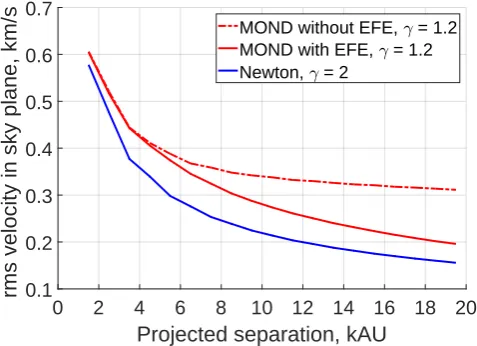
We consider the feasibility of testing Newtonian gravity at low accelerations using wide binary (WB) stars separated by_&3 kAU. These systems probe the accelerations at which galaxy rotation curves unexpectedly flatline, possibly due to Modified New-tonian Dynamics (MOND). We conduct NewNew-tonian and MOND simulations of WBs covering a grid of model parameters in the system mass, semi-major axis, eccentricity and orbital plane. We self-consistently include the external field (EF) from the rest of the Galaxy on the Solar neighbourhood using an axisymmetric algorithm. For a given projected separation, WB relative velocities reach larger values in MOND. The excess is≈20% adopting its simple interpolating function, as works best with a range of Galactic and extragalactic observations. This causes noticeable MOND effects in accurate observations of≈500 WBs, even without radial velocity measurements.

We show that the proposed Theia mission may be able to directly measure the orbital acceleration of Proxima Cen towards the 13 kAU-distantαCen. This requires an astrometric accuracy of ≈1µas over 5 years. We also consider the long-term or-bital stability of WBs with different oror-bital planes. As each system rotates around the Galaxy, it experiences a time-varying EF because this is directed towards the Galactic Centre. We demonstrate approximate conservation of the angular momentum component along this direction, a consequence of the WB orbit adiabatically adjusting to the much slower Galactic orbit. WBs with very little angular momentum in this direction are less stable over Gyr periods. This novel direction-dependent effect might allow for further tests of MOND.

Key words: gravitation – dark matter – proper motions – binaries: general – Galaxy: disc – stars: individual: Proxima Centauri

1 INTRODUCTION

The currently prevailing cosmological paradigm (ΛCDM,

Ostriker & Steinhardt 1995) is based on the assumption

that General Relativity governs the dynamics of astrophys-ical systems. This can be well approximated by Newtonian gravity in the non-relativistic regime, covering for instance planetary motions in the Solar System and galactic rota-tion curves (Rowland 2015;de Almeida et al. 2016). While the former can be well described by Newtonian gravity, this is not the case for the latter (e.g.Rogstad & Shostak 1972). Moreover, self-gravitating Newtonian disks are un-stable both theoretically (Toomre 1964) and in numerical simulations (Hohl 1971).

These apparently fatal problems with Newtonian grav-ity are generally explained by invoking massive halos of dark matter surrounding each galaxy (Ostriker & Peebles

∗Email:[email protected](Indranil Banik) [email protected](Hongsheng Zhao)

1973). Constraints from gravitational microlensing experi-ments indicate that the Galactic dark matter can’t be made of compact objects like stellar remnants (Alcock et al. 2000;

Tisserand et al. 2007). Thus, it is hypothesised to be an

undiscovered weakly interacting particle beyond the well-tested standard model of particle physics (Peebles 2017a, and references therein).

While this may be the solution, it is conceivable that Newtonian gravity does in fact break down in some astro-physical systems (Zwicky 1937). If so, this would naturally explain the remarkably tight correlation between the in-ternal accelerations within galaxies (typically inferred from their rotation curves) and the predictions of Newtonian grav-ity applied to the distribution of their luminous matter (e.g.

Famaey & McGaugh 2012, and references therein). This

mass-to-light ratios at these wavelengths (Bell & de Jong 2001;

Norris et al. 2016). These improvements reveal that the RAR

holds with very little scatter over ≈5 orders of magnitude in luminosity and a similar range in surface brightness (

Mc-Gaugh et al. 2016). Fits to individual rotation curves show

that any intrinsic scatter in the RAR must be <13% (Li et al. 2018).

In addition to disk galaxies, the RAR also holds for ellipticals, whose internal accelerations can sometimes be measured accurately due to the presence of a thin rotation-supported gas disk (den Heijer et al. 2015). The RAR ex-tends down to galaxies as faint as the satellites of M31 (

Mc-Gaugh & Milgrom 2013a). For a recent overview of how well

the RAR works in several different types of galaxy across the Hubble sequence, we refer the reader toLelli et al.(2017).

Another long-standing issue faced by ΛCDM is the highly anisotropic distribution of Milky Way (MW) satel-lites (Kroupa et al. 2005). Strongly flattened satellite sys-tems have also been identified around M31 (Ibata et al. 2013) and Centaurus A (M¨uller et al. 2018). These struc-tures are difficult to reconcile with ΛCDM (Pawlowski 2018;

Shao et al. 2018). Results from many different investigations

into this issue are summarised in tables 1 and 2 of

Forero-Romero & Arias(2018). Those authors use a different way

of quantifying asphericity but do not consider the particu-larly problematic velocity data. Even so, they find that the LG is a 3σ outlier to ΛCDM. Their section 4.4 shows that simulations including baryonic effects have a more spherical satellite distribution, worsening the discrepancy.

The basic problem is that thin planar structures suggest some dissipative mechanism. Although this is not by itself unusual, dark matter is thought to be collisionless, with the latest results arguing against the MW possessing a dark mat-ter disk (Schutz et al. 2017). Thus, the only natural way to form satellite planes is out of tidal debris expelled from the baryonic disk of a galaxy that suffered an interaction with another galaxy. This phenomenon occurs in some observed galactic interactions (Mirabel et al. 1992). Due to the way in which such tidal dwarf galaxies form out of a thin tidal tail, they would end up lying close to a plane and co-rotating within that plane (Wetzstein et al. 2007).

Such a second-generation origin of the MW and M31 satellite planes predicts that the satellites in these planes should be free of dark matter (Barnes & Hernquist 1992;

Wetzstein et al. 2007). This is due to the

dissipation-less nature of dark matter and its initial distribution in a dispersion-supported near-spherical halo. During a tidal interaction, dark matter of this form is clearly incapable of forming into a thin dense tidal tail out of which dwarf galaxies might condense. Lacking dark matter, the MW and M31 satellite plane members should have very low internal velocity dispersionsσint.

This prediction is contradicted by the high observed σ_int of the MW satellites coherently rotating in a thin plane (McGaugh & Wolf 2010). The M31 satellite plane galaxies also have rather high σ_int (McGaugh & Milgrom

2013b). This raises a serious objection to the idea that the

anomalously strong internal accelerations within galaxies are caused by their lying within massive dark matter halos.

The leading alternative explanation for these accel-eration discrepancies is Modified Newtonian Dynamics (MOND,Milgrom 1983). In MOND, the dynamical effects

usually attributed to dark matter are instead provided by an acceleration-dependent modification to gravity. The gravita-tional field strengthgat distancer from an isolated point mass M transitions from the Newtonian GM_r2 law at short range to

g = p

GM a0

r for r r_M

z }| {

s GM

a0

(1)

MOND introduces a₀ as a fundamental acceleration scale of nature below which the deviation from Newtonian dynamics becomes significant. Empirically,a0≈1.2×10

−10

m/s2to match galaxy rotation curves (McGaugh 2011). Re-markably, this is similar to the acceleration at which the classical energy density in a gravitational field (Peters 1981, equation 9) becomes comparable to the dark energy den-sityu_Λ≡ρ_Λc2_{implied by the accelerating expansion of the} Universe (Riess et al. 1998).

g2

8πG < uΛ ⇔ g . 2πa0 (2) This suggests that MOND may arise from quantum gravity effects (e.g.Milgrom 1999;Pazy 2013;Verlinde 2016;

Smolin 2017). Regardless of its underlying microphysical

ex-planation, it can accurately match the rotation curves of a wide variety of both spiral and elliptical galaxies across a vast range in mass, surface brightness and gas fraction (Lelli

et al. 2017, and references therein). It is worth emphasising

that MOND does all this based solely on the distribution of luminous matter. Given that most of these rotation curves were obtained in the decades after the MOND field equation was first published (Bekenstein & Milgrom 1984), it is clear that these achievements are successful a priori predictions. These predictions work due to underlying regularities in galaxy rotation curves that are difficult to reconcile with the collisionless dark matter halos of the ΛCDM paradigm (Salucci & Turini 2017;Desmond 2017a,b).

Although dark matter halos can be tuned to match ob-served rotation curves, this often requires the halo to be much more massive than the disk. The stability of galactic disks could then be rather different to a theory where the disk had all the mass. By generalising theToomre(1964) sta-bility condition for Newtonian disks,Milgrom(1989) showed that MOND is consistent with the stability of observed disk galaxies given reasonable velocity dispersions. This was later verified with numerical simulations, which showed that the change to the gravity law confers a similar amount of extra stability as a dark matter halo (Brada & Milgrom 1999). These simulations indicated a peculiarity of MOND in low surface brightness galaxies (LSBs), whose low accelerations were predicted to be associated with a large acceleration discrepancy. Though this was later verified (e.g. Famaey

& McGaugh 2012), the discrepancy is conventionally

Of course, these LSBs could be dynamically overheated as the Toomre condition only provides a lower limit to their velocity dispersion. This would make it difficult for LSBs to sustain spiral density waves, generally considered the expla-nation for observed spiral features in higher surface bright-ness galaxies (Lin & Shu 1964). Interestingly, LSBs also have spiral features (McGaugh et al. 1995). Assuming the density wave theory applies there too, the number of spiral arms gives an idea of the critical wavelength most unstable to amplification by disk self-gravity. Indeed,D’Onghia(2015) was able to obtain rather accurate analytic predictions for the number of spiral arms in galaxies observed as part of the DiskMass survey (Bershady et al. 2010), though this sur-vey ‘selects against LSB disks.’ Using this argument,Fuchs

(2003) found that LSB disks need to be much more massive than suggested by their photometry and stellar population synthesis models. A similar result was also reached byPeters & Kuzio de Naray(2018) using the pattern speeds of bars in LSBs, which are faster than expected in 3 of the 4 galaxies they considered.

Bars and spiral features in galaxies can be triggered by interactions with satellites (Hu & Sijacki 2018). However, without disk self-gravity, any spirals formed in this way would rapidly wind up and decay due to differential rotation of the disk (Fall & Lynden-Bell 1981, page 111). Even in a galaxy like M31, the simulations of Dubinski et al.(2008) indicate that interactions with a realistic satellite population only cause mild disk heating in excess of that which arises in the absence of satellites.

Thus, evidence has been mounting over several decades that the gravity in a LSB generally comes from its disk. This contradicts the ΛCDM expectation that it should mostly come from its near-spherical dark matter halo given the large acceleration discrepancy at all radii in LSBs. If this discrep-ancy arises due to MOND, then all galaxy disks would be self-gravitating regardless of their surface brightness.

Another consequence of the MOND scenario is that it raises the expected internal velocity dispersions of purely baryonicMW and M31 satellites enough to match observa-tions (McGaugh & Wolf 2010;McGaugh & Milgrom 2013b, respectively). MOND also greatly enhances the mutual at-traction between the MW and M31. As a result, these galax-ies must have had a close flyby 9±2 Gyr ago (Zhao et al. 2013). We conducted simulations of this flyby, treating the MW and M31 as point masses surrounded by test particle disks. The outer particles of each disk generally ended up preferentially rotating within a certain plane. If the flyby occurred in a particular orientation, then both simulated ‘satellite planes’ matched the orientations and spatial ex-tents of the corresponding observed structures (Banik et al. 2018). Their best-fitting simulation also matched several other constraints like the timing argument, the statement that the MW and M31 must have been on the Hubble flow at very early times but still end up with their presently observed separation and relative velocity (Kahn & Woltjer 1959). The calculated flyby time of 7.65 Gyr ago corresponds fairly well to the observation that the vertical velocity dis-persion of the MW disk experienced a sudden jump ≈7 Gyr ago (Yu & Liu 2018). The inner stellar halo of the MW accreted a significant proportion of its mass in a ‘major accretion event’ around that time (Belokurov et al. 2018). This strongly suggests that MOND can explain the Local

Group satellite planes and perhaps also the Galactic thick disk (Gilmore & Reid 1983) as a consequence of a past MW-M31 flyby. We are planning to test this scenario with N -body simulations similar to those conducted byB´ılek et al.

(2018).

As well as tidally affecting each other, the MW-M31 flyby would have dramatically affected the motion of LG dwarf galaxies caught near its spacetime location. The high MW-M31 relative velocity would allow them to gravitation-ally slingshot any nearby dwarf outwards at high speed, leading to some LG dwarfs having an unusually high radial velocity for their position. We did in fact find some evidence for 5 or 6 high-velocity galaxies (HVGs) like this (Banik & Zhao 2016,2017), a result also confirmed byPeebles(2017b) using his 3D ΛCDM model of the LG. We used a MOND model of the LG to demonstrate that the dwarfs reaching the fastest speeds were likely flung out almost parallel to the motion of the perturber. As a result, the HVGs ought to define the MW-M31 orbital plane (Banik & Zhao 2018c, section 3). Observationally, the HVGs do define a rather thin plane, with the MW-M31 line only 16◦out of this plane (see their table 4). Thus, we argued that the HVGs may preserve evidence of a past close MW-M31 flyby and their fast relative motion at that time.

As well as enhancing the gravity between the MW and M31, MOND should also enhance the gravity exerted by other galaxy groups. This would cause them to have a larger turnaround radius, the separation at which a galaxy has zero radial velocity with respect to the group. This turnaround radius is essentially a measure of where cosmic expansion wins the battle against the gravity of the cluster (Lee &

Li 2017). Stronger gravity would enlarge the turnaround

radius, perhaps explaining why it apparently exceeds the maximum expected in ΛCDM for the NGC 5353/4 group

(Lee et al. 2015) and three out of six other galaxy groups

(Lee 2018).

Because MOND is an acceleration-dependent theory, its effects could become apparent in a rather small system if the system had a sufficiently low mass (Equation1). In fact, the MOND radius r_M is only 7000 astronomical units (7 kAU) for a system with M = M. This implies that the orbits of distant Solar System objects might be affected by MOND (Pauˇco & Klaˇcka 2016), perhaps accounting for cer-tain correlations in their properties (Pauˇco & Klaˇcka 2017). For example, Oort cloud comets could fall into the inner Solar System more frequently as their orbits can lose their angular momentum in MOND, even without tidal effects (Section9.2). However, it is difficult to accurately constrain the dynamics of objects at such large distances.

Such constraints could be obtained more easily around other stars if they have distant binary companions. As first suggested byHernandez et al.(2012), the orbital motions of these wide binaries (WBs) should be faster in MOND than in Newtonian gravity. Moreover, it is likely that many such systems would form (Tokovinin 2017), paving the way for the wide binary test (WBT) of gravity that we discuss in this contribution. Equation1implies that this will involve orbital velocities of∼p4

GMa0= 0.36 km/s.

The WBT was first attempted by Hernandez et al.

signal was identified whereby the typical relative velocities between WB stars remained constant with increasing sep-aration instead of following the expected Keplerian decline (Hernandez et al. 2012, figure 1). However, it was later shown that their typical velocity uncertainty of 0.8 km/s was too large to draw strong conclusions about the underlying law of gravity (Scarpa et al. 2017, section 1). This work obtained accurate spectra of 60 candidate WB pairs, constraining their relative radial velocity to within ∼0.1 km/s (Scarpa

et al. 2017, table 3). Combined with parallaxes and proper

motions, these measurements showed that a handful of the candidate systems are likely genuine WBs that may be suit-able for the WBT. A few systems had a relative velocity above the Newtonian upper limit but below the MOND up-per limit, though additional follow-up work will be required to confirm the nature of these systems (Section8).

Existing data from the Gaia mission (Perryman et al. 2001) strongly suggests that many more WBs will be dis-covered (Andrews et al. 2017). The candidate systems they identified are mostly genuine, with a contamination rate of

≈6% (Andrews et al. 2018) estimated using the second data

release of the Gaia mission (Gaia DR2,Gaia Collaboration 2018a).

The separations of WB stars are small compared to typical interstellar separations of ∼1 pc. As a result, an individual WB system separated by 20 kAU should have a centre of mass acceleration towards the nearest star that is ≈100× weaker than the internal gravity of the WB. The tidal effect would be smaller still. Moreover, the effects of stars in different directions would cancel to a large extent. For the Galaxy as a whole, the overall gravitational field is still only∼a₀despite the Solar neighbourhood lying∼105_× further from the Galactic Centre than typical WB separa-tions. This implies that WBs should not be much affected by tides from the smooth component of the Galactic potential. However, the real Galaxy is not smooth as it contains many individual stars. Thus, one concern with the WBT is whether a sufficiently large fraction of WB systems survive encounters with passing field stars. Bahcall et al. (1985) estimated that the survival timescale was longer than 10 Gyr for systems separated by<31 kAU, with the survival timescale being inversely proportional to the separation.

Jiang & Tremaine (2010) also performed a detailed study

into this issue. Their figure 8 shows that a substantial frac-tion of WB systems should survive for 10 Gyr if we restrict to systems with separation below≈0.1 of their Jacobi (tidal) radius, which is 350 kAU for two Sun-like stars orbiting each other in the Solar neighbourhood (see their equation 43).

If WBs were very rare, then finding one should require us to look beyond the nearest star to the Sun, Proxima Cen-tauri (Proxima Cen). It orbits the close (18 AU) binary α Cen A and B at a distance of 13 kAU (Kervella et al. 2017). This puts the Proxima Cen orbit well within the regime where MOND would have a significant effect (Beech 2009,

2011). Given the billions of stars in our Galaxy, it would be highly unusual if it did not contain a very large number of systems well suited to the WBT. This is especially true given the high (74%) likelihood that our nearest WB was stable over the last 5 Gyr despite the effects of Galactic tides and stellar encounters (Feng & Jones 2018).

Although these works assumed Newtonian gravity, their conclusions should also be valid in MOND as it only slightly

enhances the impulse due to a stellar encounter (Figure1). The effects of the non-linear MOND gravity can cause a WB to be unstable over Gyr periods, but we find that this only affects a small proportion of WB systems in particular orientations (Section9.2).

The WBT was considered in more detail byPittordis

& Sutherland(2018), who approximated MOND using their

equation 21. This appears to significantly underestimate the gravitational attraction between the stars in a WB. In fact, the authors found a wide range of scenarios in which stars are expected to attract each other even less than under Newtonian gravity. Given the importance of the WBT, we revisit it using libraries of WB orbits based on more rig-orous MOND force calculations. These are compared with similar orbit libraries based on Newtonian gravity. We also check our numerically determined MOND forces in very wide systems using previously derived analytic results (Banik &

Zhao 2018a).

We then develop a statistical analysis procedure to quantify how many WB systems would be needed to conclu-sively distinguish between Newtonian and MOND gravity using the WBT. Our work focuses on a particular imple-mentation of MOND with the interpolating function that works best with currently available observations. Thus, our more rigorous approach complements that of Pittordis &

Sutherland(2018), who considered a wider range of modified

gravity formulations and free parameters.

After introducing the WBT in Section1, we explain how we determine the MOND gravitational attraction between the stars in each system and use this information to inte-grate the system (Section2). We then discuss our choice of prior distributions for the WB orbital parameters (Section

3). Using similar methods to obtain a Newtonian control, we compare the results using the procedure explained in Section

4. This allows us to quantify how many systems are required for the WBT, the primary result of this contribution (Sec-tion5). We then discuss measurement uncertainties in the basic parameters of nearby WB systems (Section6). Using simple analytic estimates, we discuss how the WBT might or might not work with different MOND formulations and interpolating functions (Section7). We also discuss which interpolating function is most appropriate in light of exist-ing observations, especially of rotation curves (Section7.1). The WBT can also be affected by astrophysical uncertain-ties regarding the properuncertain-ties of each system, in particular whether they contain any undetected companions (Section

8). These uncertainties could be mitigated and a much more direct version of the WBT conducted if the orbital accelera-tion were measured directly, something that may be possible with future observations of Proxima Cen (Section9). In this section, we also consider the long-term orbital stability of WB systems in the complicated time-dependent MOND po-tential. We provide our conclusions in Section10.

2 METHOD

their relative velocityv, making use of the fact that stronger gravity allows systems to be bound at a higher relative speed v≡ |v|.

One issue with the WBT is that it necessarily requires many WB systems and thus a sufficiently large survey vol-ume. Towards its edge, Gaia is unlikely to constrain line of sight distances accurately enough to know the true (3D) separationrof each system (Section6.2). However, the sky-projected separation rp would be known very accurately. To take advantage of this, Pittordis & Sutherland (2018) defined

e v ≡ v÷

Newtonianvc

z }| {

s GM

rp

(3)

e

vis the ratio ofvto the Newtonian circular velocityvc of a system with total massMif its stars are separated by a distancerp. Because their true (3D) separationr > rp, cal-culating_evin this way provides an upper limit onv÷qGM

r , a quantity which can’t exceed√2 in Newtonian gravity. In MOND, we expect the upper limit to be somewhat higher. As a result, the probability distribution of v_eshould differ between the two models, with MOND allowing for a non-zero probability that_ev >√2. This is the basis for the WBT. To forecast how this might work, we integrate forwards a grid of WB systems covering a range of masses and orbital parameters. At each timestep, we consider what would be seen by a distant (r) observer at a grid of possible viewing directions. In this way, we build up a probability distribution overrpandev. The results are compared with those of simi-lar calculations using Newtonian gravity. We then develop a statistical procedure that quantifies how easily we could dis-tinguish theevdistributions of the two theories for different total numbers of WB systems (Section 4). This addresses the question of how many systems would be needed for the WBT, thus helping observers plan its implementation.

In the near term, the WBT will be based on stars in the Solar neighbourhood. This means that our orbit integrations must take into account an important MOND phenomenon whereby the internal dynamics of a system is affected by any external gravitational field (EF), even if its strengthgext is uniform across the system. This external field effect (EFE,

Milgrom 1986) arises because MOND gravity is non-linear in

the matter distribution (Equation4). The EFE can be un-derstood intuitively by considering a system with low inter-nal accelerations that would normally show strong MOND effects. However, if the system is in a high-acceleration envi-ronment (gexta0), then the total acceleration gexceeds thea₀ threshold, making the internal dynamics Newtonian. For the WBT,gextis provided by the rest of the Galaxy. This leads to the force between two stars varying with their orientation relative to the EF direction_bgext≡|ggextext| (Banik

& Zhao 2018a). Thus, we need to consider WB systems with

a range of different angular momentum directionsbh. In gen-eral, all possible directions would need to be considered. To keep the computational cost manageable, we make the sim-plifying assumption that one of the stars is much less massive than the other. This makes the problem axisymmetric as the gravitational field is generated by a single point mass, with the other star treated as a test particle.

Such a dominant mass approximation is valid in the Newtonian regime as the linearity of this gravity theory means the mass ratio has no effect on relative acceleration. MOND gravity is also linear whengext dominates the dy-namics of a system (Banik & Zhao 2018a). In these circum-stances, the mass ratio between two stars does not affect their relative acceleration (this depends only on their total massM and separation vectorr).

Our approximation is therefore accurate both for very close and very wide systems. At intermediate separations, the force binding a WB system would be somewhat weaker if its mass were split more equally between its components

(Milgrom 2010, equation 53). This would make the_ev

distri-bution slightly more similar to the Newtonian expectation. However, we expect this to be a very small effect for rea-sons discussed in Section7.3, where we also perform some detailed calculations to help confirm this.

2.1 Governing equations

We begin by describing how we advance WB systems using the quasilinear formulation of MOND (QUMOND,Milgrom 2010). Each system is treated as a single point massM plus a test particle embedded in a uniform EFgext. QUMOND uses the Newtonian gravitational fieldg_N to determine the true gravitational fieldgby first finding its divergence.

∝ρ_{P DM}+ρ b z }| {

∇ ·g = ∇ ·



   ν

y

z }| {

g_N a0

gN 

  

where (4)

ν(y) = 1 2 +

r 1 4+

1

y (5)

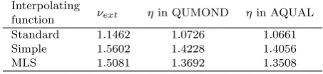
ν(y) is the interpolating function used to transition between the Newtonian and deep-MOND regimes. We use the ‘simple’ form of this function (Famaey & Binney 2005) because it fits a wide range of data on the MW and external galaxies better than other functions with a sharper tran-sition (Section 7.1). The source term for the gravitational field is∇ ·(νgN), which can be thought of as an ‘effective’ densityρcomposed of the baryonic densityρ_b and an extra contribution which we define to be the phantom dark matter densityρ_{P DM}. This is the distribution of dark matter that would be required for Newtonian gravity to generate the same total gravitational field as QUMOND yields from the baryons alone.

The Newtonian gravityg_N at positionrrelative to the central massM is given by

g_N ≡ −GMr

r3 + gN,ext (6)

The EF contributing to gN is not the true EF gext acting on the system. Rather, the important quantity is

g_N,ext, what the EF would have been if the universe was governed by Newtonian gravity. For simplicity, we assume the spherically symmetric relation betweengextandgN,ext, reducing Equation4to

gext =

ν_ext

z }| {

ν

g_N,ext a₀

!

This algebraic MOND approximation should be fairly accurate given that the Solar neighbourhood is ≈4 disk scale lengths from the Galactic Centre (Bovy & Rix 2013;

McMillan 2017). Note that this does not require the

gravita-tional field to be spherically symmetric. Instead, it requires the weaker condition that departures of g from spherical symmetry are accurately captured by applying the MOND ν function to gN, which is itself not spherically symmet-ric. This may explain why Jones-Smith et al.(2018) found that QUMOND gravitational fields in disk galaxies could be estimated rather well using the algebraic MOND approx-imation, justifying our use of Equation 7. We discuss its accuracy in Section9.3.1, finding it should work well in the Solar neighbourhood where the WBT would be conducted.

Having foundgN in this way, we use Equation4to find

∇ ·g. We then apply a direct summation procedure to∇ ·g

in order to determinegitself.

g(r) = Z

∇ ·g r0 (r−r

0

) 4π|r−r0_|3d

3

r0 (8)

As gN is axisymmetric about gbext, the phantom dark matter distribution can be thought of as a large number of azimuthally uniform rings. At points along their symmetry axisg_bext, it is thus straightforward to findgby summing the contributions from each ring. In general, the lower mass star in a system is not conveniently located alonggbextrelative to the primary star. To findgat off-axis points in a computa-tionally efficient way, we use a ‘ring library’ that storesgN due to a unit radius ring. This saves us from having to fur-ther split each ring into a finite number of elements. Instead, we can simply interpolate within our densely allocated ring library to find the gravity exerted by any ring at the point where we wish to know its contribution tog.

In this way, we can map out the gravitational field due to a point mass M embedded in a uniform EF. Using a scaling trick, we only need to do this for one value of M. This is because the only physical lengths in the problem are the MOND radiusr_M (Equation1) and the EF radiusrext wheregN =gN,ext. If we keepgN,extfixed, then it is always a fixed multiple ofa0, leading to a constant

rext

r_M. Thus, we construct a force library for some arbitrary massM= 1 and work in units whereG=a0 = 1, causing distances to be in units ofr_M and accelerations in units ofa₀.

Due to the finite extent of our grid, we can only con-sider contributions to g from the region r < rout, though we makerout sufficiently large thatgextis totally dominant beyond it. Thus, regions beyond our grid have an analytic phantom density distribution containing only a quadrupolar term (Banik & Zhao 2018a, equation 24). As explained in AppendixA, this leads to a correction ∆Φ to the potential Φ in the regionr < rout covered by our grid.

∆Φ (r, θ) = 1

5GM νextK0r 2

3 cos2θ−1

Z ∞

r_out 1

e r4 der

= GM νextK0r 2

3 cos2θ−1 15rout3

where (9)

K0 ≡

∂ Ln νext ∂ Ln g_N,ext = −

1

2 ifgN,exta0 (10) cosθ ≡ r_b·_bgext

This causes an adjustment to the gravitational field of

∆g = 2GM νext 15rout3

(r−3rcosθ_bg_ext) (11)

When considering a point wheregext is dominant, the gravity due to the star has a magnitude of≈ GM νext

r2 , mak-ing the correction to it only ∼ 1

15

r rout

3

when expressed in fractional terms. Thus, the accuracy of our results should not depend much on this correction, which should in any case be very accurate as it estimates contributions from regions with r >66.5r_M. There, g

N,ext should be should be &5000gN, allowingg_N to be considered perturbatively in the manner ofBanik & Zhao(2018a).

In the opposite extreme where the test particle gets very close to the mass, we do not need to consider the EF from the rest of the Galaxy. Thus, at distances within 0.08r_M, we assume that

g = νg_N (12)

= −νGMr

r3 (13)

At these positions, the EF (of order a0) should be &100×weaker thang_N, making it reasonable to treat the situation as isolated and neglect the EF when calculatingν. However, our algorithm will eventually slow down ifr be-comes sufficiently small. Thus, we terminate the trajectory of any particle that gets within 50 AU.

2.2 The boost to Newtonian gravity

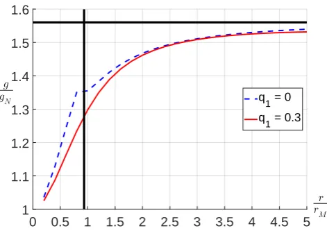
To better understand how much the gravity between two stars might be boosted by MOND effects, we determine the angle-averaged ratioηbetween the MOND and Newtonian radial gravity at different separations.

η(r) = 1 4π

Z π

0

gr(r, θ)

g_N,r(r)2πsinθ dθ (14)

In very widely separated systems, the total acceleration is dominated by the EF rather than self-gravityg. In this limit, we can obtain gr analytically (Banik & Zhao 2018a, equation 37).

gr = gN,rνext

1 +K0 2 sin

2 θ

(15)

Substituting this into Equation14yields

η = νext

1 +K0 3

(16)

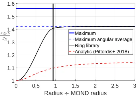
The angle-averaging makesηa good guide to how much gravity would be boosted by MOND effects in a system with known separation relative to its MOND radius. In Figure1, we compare the numerically determined value ofηat differ-ent radii with this EF-dominated expectation.

For completeness, we note that the maximum value of gr

g_N,r requires not only that the EF dominate (gN,ext g) but also that the angleθ= 0 orπ(Equation15). Thus, the MOND boost to the self-gravity of the system is limited to

gr

0 0.5 1 1.5 2 2.5 3

Radius MOND radius

1 1.1 1.2 1.3 1.4 1.5 1.6

Maximum

Maximum angular average Ring library

Analytic (Pittordis+ 2018)

Figure 1.The azimuthally averaged quantityη(Equation14) for our QUMOND force library as a function of separation between the stars in a wide binary, assuming one of the stars dominates the system (solid black curve). Our results apply to systems of any mass, as long as distances are scaled to its MOND radius rM (Equation1) and the EF from the rest of the Galaxy has the Solar neighbourhood value (Equation7). We also show the result obtained byPittordis & Sutherland (2018) using their equation 21 (dashed red curve). The EF dominates the dynamics of suf-ficiently widely separated systems (right of black vertical line). Analytic calculations in this regime show thatη asymptotically reaches the value given by Equation16 (dashed blue line). For systems aligned with the EF, the maximum ratio of MOND and Newtonian gravity is given by Equation17(solid blue line).

2.3 Orbit integration

2.3.1 Initial conditions

To investigate a range of WB orbital semi-major axesaand eccentricitiese, we first need to define what these quantities mean in MOND. To generalise their definitions for modified gravity theories while remaining valid in Newtonian gravity, we follow the work ofPittordis & Sutherland(2018, section 4.1).ais defined as the orbital separationrat the point in the orbit where the speedvsatisfies

v = √−r·g (18)

There will be two points in the orbit which satisfy this equation. Either point can be used as they both have the samer. These points are also used to defineeaccording to

e = |rb·vb| (19)

We use the usual Galactic Cartesian co-ordinates withx_b

towards the Galactic Centre,zbtowards the North Galactic Pole andy_b=z_b×x_bso that the co-ordinate system is right-handed. As a result, ybpoints along the direction in which the Solar neighbourhood rotates around the Galaxy.

The massive component of each WB is assumed to re-main at the origin. We start the other component at the position (0, a,0) and use Equation18to setv. Equation19

is used to fix the component ofvalong the radial direction.

vy = v e (20)

The remaining tangential velocity vtan must have a magnitude ofv√1−e2 _{and lie within thexz-plane. We}

ad-just the direction ofvtan in order to change the orbital pole b

h∝r×v, thereby investigating a range of possible angles betweenhb and g_bext = xb. Due to the axisymmetry of the problem, it is only necessary to consider orbital poles along a single great circle containing _bgext. In our setup, this is achieved by considering all possiblebhwithin thexz-plane. As MOND orbits are not closed, we can start our simulations anywhere in the plane orthogonal toh. Thus, it is always valid to start on they-axis.

When running Newtonian control simulations to com-pare with the MOND ones, the orbit is closed. However, its conserved orientation within the orbital plane has no effect on the internal dynamics of the system as the force law is not angle-dependent. Thus, we can use the same setup for our Newtonian runs, though these benefit from a number of simplifications compared to the MOND runs.

2.3.2 Advancing the system

We evolve our WB systems forwards using our dimensionless force libraries (Section 2.1). This requires us to scale co-ordinates down by the value ofrM appropriate to the mass M of the system we are considering (Equation1). We then use interpolation to estimate the relative acceleration at the instantaneous separationr of the WB system. This is used to advancerwith the fourth-order Runge-Kutta procedure. As the dynamical time should be similar to what it would be in Newtonian gravity, we use an adaptive timestep of

dt = 0.01 r

r3

GM (21)

We evolve each system forwards until it completes 20 revolutions, representing a rotation angle of 40π radians. To determine the rotation angle over each timestep, we use the dot product between the initial and final directions of

b

r. The algorithm is accelerated by using a small angle ap-proximation at one order beyond the leading order term, thereby minimising the use of computationally expensive inverse trigonometric functions.

As the MOND potential is non-trivial, it is possible forr to reach very small or very large values compared to its initial value. We therefore terminate trajectories when r <50 AU or whenr >100 kAU. We assign zero statistical weight to the parameters which cause the system to ‘crash’ or ‘escape’ in this way. The upper limit is chosen based on the observed 270 kAU distance of Proxima Cen (Kervella

et al. 2016). We expect that WBs with separations exceeding

about half this would be so widely separated that nearby stars could unbind the system. The lower limit is chosen to avoid spending excessive amounts of computational time on systems which would likely lose significant amounts of energy through tides, thus taking the orbital parameters outside the region of interest for the WBT. For our purposes, it is not important to know whether these systems would actually undergo a stellar collision or merely settle into a much tighter binary (Kaib & Raymond 2014).

Section9, we consider how this affects the long-term evolu-tion of WBs. We also show that our results should not differ much if we had advanced our simulations for 5 Gyr rather than 20 revolutions and allowedgbextto rotate (Figure15).

2.3.3 Recording of results

Due to the large number of WB parameters we explore, it is difficult to store all the information available from our trajectory calculations. Moreover, we are not interested in doing so as the observations only constrain certain features of the orbits, and even then only in a statistical sense given that we see a very small fraction of the orbit. Thus, we use our simulated trajectories to obtain the joint probability distribution of the main observable quantitiesrpandev.

To do this, we create a 2D set of bins in rp andev. At each timestep and for each viewing angle (Section3.5), we increment the probability of the corresponding (rp,ev) bin by the duration of the timestep multiplied by the relative probability of that particular viewing angle. Afterwards, we normalise the final probability distribution over (rp,ev). If a trajectory crashes or escapes, then we assign zero probability to that particular combination of model parameters.

Our approach is valid as few WBs are destroyed on an orbital timescale (Section8.1). As this is much shorter than a Hubble time, we assume the creation timescale of WBs is also much longer than an individual orbit. This leads to the (rp,v) distribution remaining steady over many orbits.e

3 PRIOR DISTRIBUTIONS OF BINARY

PARAMETERS

For the WBT, we need prior distributions for the various system parameters. The ones we consider are the semi-major axis a and eccentricity e (defined in Section 2.3.1), total system mass M, the angle θ betweenhb and

b

gext and two angles governing the direction from the WB system towards the observer, assumed to be very far from the system. To allow easy investigation of different priors without rerunning the orbital integrations, we record the resultingP(rp,ev) for the full grid of M, a and e. We do not store results for different angle parameters because we assume that they all have an isotropic distribution, allowing us to marginalise over them prior to recording the results (Sections 3.4 and

3.5).

3.1 Eccentricity

Following section 4.1 ofPittordis & Sutherland (2018), we assume the WB orbital eccentricity distribution P(e) has the linear form

P(e) = 1 +γ

e−1 2

(22)

The anti-symmetric factor e−1 2

is required to ensure the normalisation condition R1

0 P(e)de = 1. We assume that the constantγ= 1.2 for the MOND case (Tokovinin &

Kiyaeva 2016). To avoid negative probabilities,−26γ62.

When comparing with Newtonian gravity, it is necessary to also defineγN, the corresponding value ofγfor the Newto-nian model. If the WBT yielded a positive result for MOND,

Variable Meaning Prior range

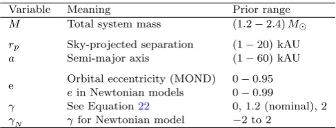
M Total system mass (1.2−2.4)M

rp Sky-projected separation (1−20) kAU

a Semi-major axis (1−60) kAU

e Orbital eccentricity (MOND) 0−0.95 ein Newtonian models 0−0.99

γ See Equation22 0, 1.2 (nominal), 2 γN γfor Newtonian model −2 to 2

Table 1.Our prior ranges on wide binary orbital parameters. Although we extract probabilities for sky-projected separations rp up to 100 kAU, we assume that the WBT would be based on systems withrp= (1−20) kAU to minimise contamination by interlopers (at highrp) and avoid nearly Newtonian systems (at lowrp). As the Newtonian versions of these simulations are much faster, we use a higher resolution and wider range in e. For each value ofγ, we try all possible values of γN and take the value which minimises the detection probability (Section4). Qualitatively, this yields a Newtonianevdistribution most similar to the MOND one.

then astronomers would almost certainly try to fit the data with Newtonian gravity by adjustingγ_N. In general, trying to match the high ev values expected in MOND requires Newtonian models with a large e as only such orbits can getv_eto significantly exceed 1. Giving a higher probability to higheorbits implies a higherγ_N.

As we do not a priori knowγ_N, we need to let it vary when estimating how easily the Newtonian and MOND _ev distributions could be distinguished using the method de-scribed in Section 4. The ‘best-fitting’ γN is that which makes this task the most difficult. This requires us to con-sider all possible values for γN. Although γN can be neg-ative, this would further reduce the probability of high e orbits, likely worsening the agreement with observations of a MOND universe. Thus, we assume the optimalγ_N lies in the range (0,2). Where it is clear that this is not the case because negativeγN is preferred, we consider the full range of physically possible values forγ_N (Section5).

As the correct value ofγ is not known either, we con-sider the three cases of 0 (a flat distribution), 1.2 (Tokovinin

& Kiyaeva 2016) and 2. These were the three cases

consid-ered byPittordis & Sutherland(2018), as discussed in their section 2.1. Each time, we need to repeat our search for the best-fitting γ_N. Our procedure is thus fully deterministic, avoiding uncertainties due to the use of random numbers.

3.2 Semi-major axis

To constrain the semi-major axis distributionP(a), we use the observedP(rp) distribution (Andrews et al. 2017, sec-tion 6.2).1 Similar results were obtained byL´epine & Bon-giorno(2007), though with a slightly smaller break radius of 4 kAU.

P(rp)drp ∝ (

rp−1drp ifrp65 kAU rp−1.6drp ifrp>5 kAU

(23)

Model γ α β a_break Newton

−2 0.8 1.63 5.14 0 0.92 1.66 5.16

2 1 1.63 4.59

MOND

0 0.88 1.96 7.39 1.2 0.92 1.95 7.39 2 0.95 1.94 7.41

Table 2.Parameters governing our prior distribution of wide bi-nary semi-major axes in different Newtonian and MOND models (Equation24). These are chosen to best reproduce the observed distribution of sky-projected separations (Equation23).

To match these results, we use a broken power law for P(a) with the break ata=a_break.

P(a)da ∝

a−αda ifa6a_break a−βda ifa>abreak

(24)

We considerain the range (1−60) kAU, though with reduced resolution beyond 25 kAU. The lower limit of 1 kAU is chosen because the rather gradual interpolating function we adopt (Famaey & Binney 2005) implies that departures from Newtonian gravity decay rather slowly as the accel-eration rises above a₀. Moreover, tighter orbits are more common (Andrews et al. 2017), so they might contribute something to the WBT even if they are not much different from Newtonian expectations.

Due to our imposed maximum separation of 100 kAU, orbits witha >60 kAU are often terminated early and do not contribute any statistical weight to the WBT. Such large orbits are in any case unlikely (Andrews et al. 2017). More-over, we only expect to perform the WBT using systems withrp620 kAU, making it not particularly important to consider orbits for whichais much larger.

As we are not a priori sure which range inrpwill work best for the WBT, our algorithm is allowed to find the opti-mal range within the (1−20) kAU range we allow (Section

4). In Section5, we will see that the WBT does not benefit from systems with rp . 3 kAU, justifying our decision to neglect WBs witha <1 kAU.

To determine the best fitting values ofα,βanda_break, we try a grid of models in all three parameters. For each combination, we find P(a) using Equation 24. We then marginalise overv_eand the other model parameters to obtain a simulated P(rp). This is done over kAU-wide bins in rp over the range (2−20) kAU, thus minimising edge effects from our lack of models witha <1 kAU and our truncation of orbital separation at 100 kAU. We then normalise our simulated distribution to yield the relative frequency of WB systems in each rp bin. This is compared with the corre-sponding observed quantity using aχ2 _{statistic. We select} whichever combination (α, β, abreak) yields the lowestχ

2 . This procedure relies on knowing the eccentricity dis-tributionP(e). For the Newtonian models, we try a range of possible distributions parameterised by γ_N (Section

3.1). Thus, we need to repeat our grid search through (α, β, a_break) for each value ofγ_N.

As a first approximation, we can assume that these parameters are equal to the values governing the observed P(rp). This would giveα= 1,β= 1.6 andabreak= 5 kAU (Equation 23). Our results indicate that this estimate is reasonably accurate regardless of the adoptedγ, especially

1 1.2 1.4 1.6 1.8 2 2.2 2.4

Binary system total mass, M

0 0.02 0.04 0.06 0.08 0.1 0.12 0.14

Probability

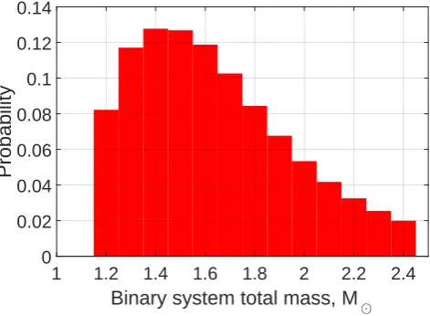
Figure 2.Our adopted prior distribution P(M) for the total massMof WB systems in the Solar neighbourhood (Section3.3).

for the Newtonian model (Table2). We are always able to match the observedP(rp) distribution to within a root mean square (rms) scatter of 0.3% over the range that we try to fit.

Based on our results, we suggest that future work could approximate P(a) = P(rp) in order to avoid one of the most computationally intensive parts of our algorithm. This works especially well for the Newtonian model. Even if this approximation is not made, it should be possible to speed the process up by searching more efficiently through differ-entP(rp) distributions of the form given in Equation 23. For example, a gradient descent method could be used or a multigrid approach tried that successively zooms into the region around the model with the lowestχ2.

3.3 Total system mass

Due to the complexity of MOND, our orbit integrations make the simplifying assumption that all of the mass M in each WB system is contained within one of its stars. The dependence of WB dynamics on the mass ratio is discussed in Section7.3, where we show that the effect is small (though not zero like in Newtonian gravity). As a result, we need a prior distribution forM.

To construct this priorP(M), we assume the stars in each WB have independent masses (Belloni et al. 2017, figure 2). This leaves us with the simpler task of obtaining the mass distribution _ep(m) for isolated stars. We assume that this follows a broken power law.

e

p(m)dm ∝

m−2.3_{dm ifm}

6M

m−4.7dm ifm>M (25)

Here,mis the mass of an individual star. We use a high-mass slope of−4.7 (Bovy 2017, equation 17) and a low-mass slope of−2.3 (Kroupa 2001, equation 2). The resultingp_e(m) is used to obtainP(M) by integration.

P(M)dM =

Z M−mmin

mmin e

p(m)p_e(M−m)dm (26)

assume that the WBT will not use stars withm < mmin= 0.55Mbecause of their faintness. Due to the steeply declin-ing stellar mass function above M, we only consider WB systems withM in the range (1.2−2.4)M. The resulting P(M) is shown in Figure2.

In Newtonian gravity, the scale invariance of the force law implies that M is irrelevant for the (rp,v) distributione once a and e are fixed. This allows our Newtonian orbit library to consider just one value forM. We arbitrarily set this to 1.5M.

The mass of each WB system has only a small effect on its expected orbital velocity. This is because MOND effects arise at smaller separations in a lower mass system, counter-acting the tendency of these systems to rotate slower. Using Equation3to estimate the circular velocityvcat the MOND radiusr_M (Equation1), we see that

vc(rM)∝ 4

√

M (27)

Consequently, systems with total massM = 1M in-stead of 2M would rotate only 16% slower at the point where MOND effects start to become significant. This sug-gests that the WBT could benefit from much better statistics if it uses observations of lower mass systems. This would also allow contamination to be reduced via a tighter cut on the projected separation, as MOND effects would arise closer in (Equation1).

In the short term, the most serious problem with this is that lower mass stars are much less luminous (e.g.Mann

et al. 2015). In the long run, this can be addressed with the

use of larger telescopes and longer exposures. Using more common systems also makes it more likely that there would be a suitable background object within the same field of view whose true parallax and proper motion can be neglected, making it useful for calibration.

3.4 Orbital plane

Due to the presence of a preferred directiong_bextinduced by the EF, the behaviour of a WB system will depend some-what on the orientation of its orbital polebhwith respect to

b

g_ext. As the WB orbital period is expected to be at most a few Myr1, we do not expect bgext to rotate significantly during a few WB orbits. Combined with our assumption that each WB system is dominated by one of its stars, this leads to an axisymmetric potential. Consequently, the only physically relevant aspect ofbhis its angleθwith_bg_ext.

We take this into account by considering a grid of pos-sible θ whose prior distribution P(θ) is assigned based on the assumption thatbhis isotropically distributed.

P(θ)dθ = 1

2sinθ dθ (28) We only consider angles θ 6 π

2 as larger angles are equivalent to a WB with a lowerθbut with its initial velocity reversed. Because gravitational problems are time reversible, this should not affect WB characteristics like its average orbital velocity. Such properties are thus expected to be the same forθ→π−θ.

1 _{using Kepler’s Third Law for stars similar to the Sun and a} separation below 20 kAU

In the long term, the EF on each WB changes with time as it rotates around the Galaxy. However, we do not expect this to affect our results very much because the Galactic or-bit is much slower than the WB oror-bit. As a result, the initial distribution ofθis likely preserved (Figure17), maintaining a nearly isotropicbhdistribution. This issue is discussed fur-ther in Section9.2, where we show that the distribution in rp and ev is nearly the same whether the orbit of Proxima Cen is integrated for just 20 revolutions with a fixed EF or over 5 Gyr in a time-varying EF (Figure15). This is because each WB system is expected to haverbgo through a wide range of directions relative to the EF such that the gravity between its stars follows an angular average. In any case, even an EF-dominated system in the Solar neighbourhood should not have a self-gravity that depends very much on its orientation relative to the EF (using K0 = −0.26 in Equation15shows that the force is affected at most 9%).

3.5 Viewing angle

Gaia observations are not expected to yield all six phase space co-ordinates for most WB systems it discovers. In par-ticular, the line of sight separation between the stars would generally not be known as accurately as the other observ-ables (Pittordis & Sutherland 2018), with our calculations suggesting an accuracy of∼80 kAU (Section6.2). The radial velocity difference between the stars may also be difficult to determine at the∼0.1 km/s accuracy required for the WBT. In addition to accurate spectra, this also requires knowledge of the difference in convective blueshift corrections between the stars (Kervella et al. 2017). In the short run, this makes it inevitable that what we infer about each system will depend on its orientation relative to our line of sight towards it.

To take this into account, at each timestep of our WB orbital integrations, we consider a 2D grid of possible direc-tionsnbin which the observer lies relative to the WB system. Assuming the observer is much more distant than the WB separationr, we determinerpusing

rp = |r−(r·nb)nb| (29)

We use this in Equation3 to find_ev, assuming masses are known regardless of the viewing angle as these should be determined from luminosities of nearly isotropic stars (Section6.3). We then increment the appropriate (rp,ev) bin by the fraction of the full 4πsolid angle represented by each

b

n, assuming this has an isotropic distribution. This should be valid out to the≈150 pc distance relevant for the WBT as the MW disk scale height is larger (Ferguson et al. 2017, figure 7).

3.6 External field strength

We take the EF to point towards the Galactic centre and have a magnitude sufficient to maintain the observed Local Standard of Rest (LSR) speed of vc, = 232.8 km/s, as-suming the Sun isR = 8.2 kpc from the Galactic centre

(McMillan 2017). Gaia DR2 remains consistent with these

parameters (Kawata et al. 2018).

function altersg_N,ext. We use the simple form of this func-tion for reasons discussed in Secfunc-tion7.1.

In principle, Equation7is only valid in spherical sym-metry and is thus invalid near the MW disk and its resulting vertical force. However, this is expected to be rather small in the Solar neighbourhood because we are ≈4 disk scale lengths from the Galactic Centre (Bovy & Rix 2013). We consider the accuracy of this algebraic MOND approxima-tion in Secapproxima-tion9.3.1. There, we show that the local value of νextshould be affected <1% by the vertical gravity due to the MW disk.

4 THE DETECTION PROBABILITY

To forecast the feasibility of the WBT, we need to obtain and compare theP(_ev) distributions expected in Newtonian and MOND gravity. We obtain these distributions by marginal-ising over WB parameters using the prior distributions out-lined in Section3. As our prior onais already chosen to get an appropriate posterior distribution for rp (Section 3.2), marginalising overrpis very simple. For consistency, we use the numerically determinedP(rp) rather than the observed distribution, though the differences are very small (rms error .0.3%).

To compare the Newtonian PN(ev) with the MOND PM(_ev), we use an algorithm that we make publicly available as it can be used to forecast the distinguishability of any two probability distributions.1 This provides a quantitative estimate of how easily we can distinguish the two theories usingN well-observed WB systems in different ranges ofrp contained within the interval (1−20) kAU. In this way, we quantify how many such systems would be needed for the WBT. The actual number is likely to be somewhat larger due to observational uncertainties (Section 6) and various systematic effects (Section8). Moreover, not all WB systems will be suitable for the WBT.

Our approach is to find the likelihood that observations drawn fromPM(ev) are inconsistent with expectations based onPN(ev). Suppose we haveN= 100 systems and are inter-ested in the number n of them which have _ev >1.2. If we expect n = 9.7 in Newtonian gravity but a larger number in MOND, then we begin by finding the maximum value of n at the 99% confidence level according toPN(ev). For-mally, this valuenmaxis the smallest integer which satisfies P(n6nmax)>0.99. Due to the discreteness of WB sys-tems, P(n) follows a binomial distribution whose parame-ters are (100,0.097) in this example.

This leads to the conclusion that the Newtonian model could be used to explain any observedn6nmax= 16. We then find the likelihood that n > nmax if the observations correspond to a MOND universe. We call this likelihood the detection probabilityPdetectionof MOND relative to Newto-nian gravity for the adopted prior distributions, (rp,_ev) range and number of systems used.

If we use a_evrange in whichPM(_ev) has less probability thanPN(ev), we reverse the logic outlined above. Thus, we find the 99% confidence levellowerlimit ofPN(v). We then_e

1 _{Algorithm available at:MATLAB file exchange, code 65465}

determine the likelihood thatnis even smaller if the obser-vations are drawn from PM(_ev). In practice, this situation should not arise because we expect the WBT to work best by focusing on high values of_evwhich are more common in MOND. Even so, our analysis is not a blind search for dis-crepancies with the Newtonian model but a more targeted search for discrepancies in the direction that would arise if MOND were correct. Blind analyses should also be con-ducted, especially if neither model describes the observations well.

When conducting our analysis, we try all possible rect-angular regions in (rp,ev) space to see which one maximises Pdetection. We expect the algorithm to use the full range of rpavailable to it (Table1), but it is not clear a priori exactly which range ofevwill work best. This is because both models predict nearly 100% of systems within a very wide_evrange. If a very narrow range were used instead, it is quite possible that this has some probability of arising in MOND but no chance in Newtonian gravity. This is good for the WBT in the sense that a detection within the adopted_evrange would constitute very strong evidence for MOND. However, even in MOND, it may be very unlikely to observe such a system. This would lead to a lowPdetection. Thus, some intermediate range ofveis expected to be most suitable for the WBT. Our discussion so far suggests a range from the high end of the Newtonianevdistribution to the upper limit of the MOND distribution.

Although we are a priori unsure exactly which_evrange works best, it is clear that its lower limit_evminshould not be set above the maximum possible_evin the Newtonian model. This is because raising_evminabove this value does not further reduce the already zero probability of finding a Newtonian WB system withev >evmin. However, increasingevmin does reduce the probability of finding a system like that if gravity were governed by MOND. Thus, raisingveminabove 1.42 can only ever reducePdetection. For this reason, we restrict the algorithm to only consider_evmin61.42.

The upper limit on_ev is not restricted apart from the basic requirements to exceed_evminand to lie below the max-imum of 1.68 which arises in our MOND models.2In theory, selecting a larger value will not affectPdetection. However, in the real world, this would lead to additional sources of contamination that could hamper the WBT (Section8).

If the data give any hint of a MOND signal, this will be highly controversial and immediately raise many obser-vational and theoretical questions. On the theory side, as-tronomers would inevitably try a differentγ_N, thus changing the eccentricity distribution for the Newtonian model. In particular, higher values of γ_N would increase the weight given to highly eccentric orbits, making it more likely that_ev significantly exceeds 1. In future, it may be possible to pre-dict the Newtonian eccentricity distribution. As this is not currently possible, we use the most conservative case where the value ofγ_N is that which makes the WBT as difficult as possible. We find this by trying a grid of possible values for γ_N, each time recordingPdetection. WhicheverγN yields the lowestPdetectionthen setsPdetectionfor that particular value ofN. In this way, we quantify how well the WBT can be

0 0.2 0.4 0.6 0.8 1 1.2 1.4 1.6 1.8 0

0.005 0.01 0.015 0.02 0.025 0.03

Probability

Newton, = -2 Newton, = 0 Newton, = 2 MOND, = 0 MOND, = 1.2 MOND, = 2

0 0.2 0.4 0.6 0.8 1 1.2 1.4 1.6 1.8 0

0.002 0.004 0.006 0.008 0.01 0.012 0.014 0.016 0.018 0.02

Probability

Newton, = -2 Newton, = 0 Newton, = 2 MOND, = 0 MOND, = 1.2 MOND, = 2

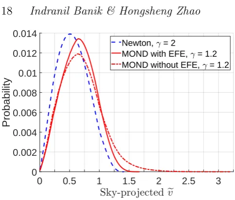
Figure 3. Distributions of the scaled WB relative velocity ev (Equation3) in Newtonian and MOND gravity, using the prior distributions from Section3. We only consider WB systems with sky-projected separationrp= (1−20) kAU. Different eccentric-ity distributions are shown by varying γ (Equation22). Notice howγ andγ_N do not much affect the results forev&1.1.Top: Using the full 3D relative velocity in the definition ofev(Equation 3).Bottom: Using the sky-projected velocity only.

pected to work for different values ofN and different model assumptions, both for Newtonian gravity and for MOND.

5 RESULTS

We begin by showing the_evdistributionsP(_ev) for the Newto-nian and MOND models under various different assumptions aboutγ(Figure3). The distributions are rather insensitive toγ(Equation22) in the region_ev&1.1, a result also evident from figure 2 of Pittordis & Sutherland (2018). Clearly, a much larger fraction of WB systems have such a high evin MOND than in any plausible Newtonian model.

It may initially seem surprising thatγN does not much affect the Newtonian _ev distribution for _ev & 1.1. After all, such high values of_evare impossible for nearly circular orbits but quite possible for elliptical orbits. However, a highly el-liptical orbit spends the majority of its time near apocentre, where _ev is very low. Consequently, such an orbit will not contribute much probability to the regionv >_e 1.1. This is

0 50 100 150 200 250 300

Number of systems

0 0.2 0.4 0.6 0.8 1

Detection probability

Full 3D velocity, = 0 3D velocity, = 1.2 3D velocity, = 2

Sky-projected velocity only, = 0 Sky-projected velocity, = 1.2 Sky-projected velocity, = 2

Figure 4.The probability Pdetection of detecting a significant departure from Newtonian expectations if the underlyingev dis-tribution follows the MOND model. The method used is explained in Section4. For each value ofγ, we choose the value ofγN which minimises Pdetection. This ‘best-fitting’ γN is≈0.5 below the value ofγadopted for the MOND model. Thus, we consider all possibleγ_N for the models whereγ= 0.

why Newtonian models with any value ofγN can never per-fectly mimic a modified gravity theory with a higher circular speed (Equation18).

In Section2.2, we used Equation 16 to estimate how much MOND would typically enhance the gravity binding a WB if the EF were dominant. This is a reasonable approx-imation towards the upper limit of the WB separations we consider. Therefore, we expect that

e v 6

s

2

1 +K0 3

(30)

In the Solar neighbourhood, this suggests that the MOND_evdistribution extends up to 1.68. This is indeed the upper limit of our much more rigorously determined MOND

e

vdistributions (Figure3).

So far, we assumed that the WBT requires the full 3D relative velocityvof each system. However, Gaia is expected to release proper motions for a large number of stars before there is time to follow them up and take accurate radial velocity measurements. Moreover, these can be hampered by uncertainties in convective blueshift corrections (Kervella

et al. 2017, section 2.2). Thus, we redo our analysis using

only the sky-projected velocity, which we find in a similar way torp(Equation 29). The resulting evdistributions are shown in the bottom panel of Figure3.

Having obtained Newtonian and MOND_evdistributions, we compare them using the method explained in Section

4. This allows us to quantify the detectability of MOND effects for different numbers of WB systems. Our results show that the WBT should be feasible with a few hundred well-observed systems (Figure4).

0 50 100 150 200 250 300

Number of systems

0 0.2 0.4 0.6 0.8 1

Detection probability

Full 3D velocity, r

p 40 kAU

Full 3D velocity, r_p 20 kAU Full 3D velocity, r_p 10 kAU Velocity on sky, r

p 40 kAU

Velocity on sky, r_p 20 kAU Velocity on sky, r

p 10 kAU

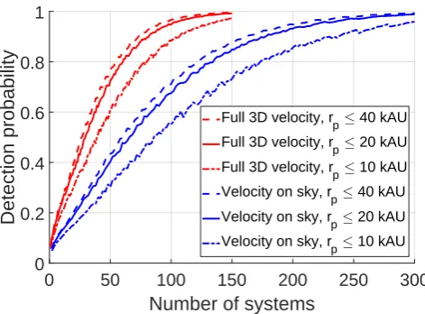
Figure 5.Similar to Figure 4 for the caseγ = 1.2, but with different upper limits onrp. Probabilities are normalised to the number of systems with rp between 1 kAU and the maximum considered for each curve, avoiding changes toPdetection due to a different number of WB systems in each range ofrp(Figure6). Once rp & 10 kAU, changing the outer limit onrp has only a small effect on our analysis because the MOND boost to gravity is limited by the Galactic external field (Figure1).

>16/100 systems in that parameter range under the MOND model. If N is raised slightly, then the chance of getting 615 systems like that might drop to 98.9% in the Newto-nian model. As this is below 99%, we would be forced to consider that Newtonian gravity can explain the existence of 616 systems in the selected parameter range at the adopted 99% confidence level. This causes a sudden drop inPdetection because this is now based on observing>17 systems in the chosen parameter range rather than the previous>16. Con-sequently, althoughPdetectiongenerally increases withN, it occasionally decreases because it is impossible to exactly maintain a fixed confidence level with a finite number of data points.

When using the full 3D relative velocity and an interme-diate value forγof 1.2, our calculations show that the WBT is best done by considering systems with ev > 1.05±0.02, with the scatter arising from discreteness effects. As ex-pected, the analysis prefers not to impose an upper limit on_ev, thus considering systems with_evall the way up to the maximum value of 1.68 which arises in our MOND simula-tions. The probability of finding a WB system in this range is≈16±2% for the MOND model but only≈4.5±1% for the Newtonian model.

If using sky-projected velocities only, it becomes best to consider the range_ev >0.97±0.02 because the sky-projected velocity is generally smaller than the full velocity. The prob-ability of finding a WB system in this range is≈9±1% for the MOND model but only ≈3±1% for the Newtonian model.

As well as giving guidance on what_evrange is best for the WBT, our algorithm also provides information about the bestrprange. At the lower limit, the algorithm generally prefers to use 3 kAU even though it could have extended this down to 1 kAU. The fact that it does not means that the

0 5 10 15 20 25 30 35 40 45 50 55 60

Sky-projected separation r

p

, kAU

0 0.1 0.2 0.3 0.4 0.5 0.6 0.7 0.8 0.9 1

Fraction of systems with lower r

p

Figure 6.The cumulative probability distribution ofrpfor WB systems with rp = (3−60) kAU, according to the empirically determined Equation23.

WBT is worsened by including such systems, presumably because they are very nearly Newtonian.

At the upper limit, the algorithm behaves as expected by preferring to use systems with rp up to the maximum of 20 kAU that we allow. This shows that the WBT would benefit from including even more widely separated WBs if they could be accurately identified and their slower relative velocities accurately measured. The work ofAndrews et al.

(2018) suggests that this may be feasible (they went up to 40 kAU).

To investigate how much this would help the WBT, we repeat our analysis with the upper limit onrp raised to 40 kAU but fix γ at our nominal value of 1.2. To avoid the increased number of WB systems automatically improving Pdetection, we normalise our probability distribution to the number of WB systems whoserp= (1−40) kAU.

The increased range in rp has only a small effect onPdetection (Figure 5). In fact, our algorithm sometimes prefers not to use this extra information, instead restricting itself torp <37 kAU to exploit the discrete nature of the data. Clearly, there is only a marginal benefit to doing the WBT with systems that have rp 6 40 kAU instead of 20 kAU.

This is also evident from Figure1, where we see that the MOND boost to gravity does not increase much for systems more widely separated than their MOND radius (Equation

1). As this is only 11 kAU for the heaviest systems we con-sider (2.4M), it is not very helpful to consider systems which are much more widely separated.

Although the MOND effect is not much enhanced by going out to 40 kAU instead of 20 kAU, this would increase the number of systems available for the WBT. The way in which this occurs can be quantified based on existing observations of the WB rp distribution (Section 3.2). By integrating Equation23and considering only systems where rp = (3−60) kAU, we get the cumulative distribution of rp shown in Figure6. This shows that the number of WB systems is unlikely to increase much as a result of increasing the upper limit onrpfrom 20 kAU to 40 kAU.