Eigenvalue Computation of Regular 4th Order Sturm Liouville Problems

(1)

https://www.scirp.org/journal/am ISSN Online: 2152-7393

ISSN Print: 2152-7385

DOI: 10.4236/am.2019.109056 Sep. 26, 2019 784 Applied Mathematics

Eigenvalue Computation of Regular 4th Order

Sturm-Liouville Problems

*

Ahmad Alalyani

Al Baha University, Al Baha, KSA

Abstract

In this paper we present and test a numerical method for computing eigen-values of 4th order Sturm-Liouville (SL) differential operators on finite inter-vals with regular boundary conditions. This method is a 4th order shooting method based on Magnus expansions (MG4) which use MG4 shooting as the integrator. This method is similar to the SLEUTH (Sturm-Liouville Eigenva-lues Using Theta Matrices) method of Greenberg and Marletta which uses the 2nd order Pruess method (also known as the MG2 shooting method) for the integrator. This method often achieves near machine precision accuracies, and some comparisons of its performance against the well-known SLEUTH software package are presented.

Keywords

4th Order Sturm-Liouville Problem, Magnus Methods (MG4), Regular Boundary Conditions

1. Introduction

In this paper1_{we consider the self-adjoint differential operators which arise from}

the 4th order differential equation

( )

( )4

_{( )}

₍

_{( ) ( )}

₎

_{( ) ( )}

_{( )}

,

L y =y x − s x y x′ ′+q x y x =

λ

y x a≤ ≤x b (1)

when separated, self-adjoint boundary conditions are imposed at each of the two regular endpoints x=a and x=b.

We make the assumptions: 1) q x

( )

is continuous on

[ ]

a b, .

2) s x

( )

and s x′

( )

are continuous on

[ ]

a b, .

*2010 Mathematics Subject Classication 34L15; 34L16; 65L15; 70J50.

1_{The content of this paper is related to my Ph.D. dissertation}_[1]_.

How to cite this paper: Alalyani, A. (2019) Eigenvalue Computation of Regular 4th Order Sturm-Liouville Problems. Applied Mathematics, 10, 784-803.

https://doi.org/10.4236/am.2019.109056

Received: July 21, 2019 Accepted: September 23, 2019 Published: September 26, 2019

http://creativecommons.org/licenses/by/4.0/

(2)

DOI: 10.4236/am.2019.109056 785 Applied Mathematics

3) −∞ < < < ∞a b .

Under these assumptions both endpoints a and b are regular endpoints. The most general separated, self-adjoint boundary conditions which can be imposed at x=a and x=b are

( )

( ) ( ) ( )

( )

1

1 2

2

0 0

l y y a y a s a y a

A A

l y y a y a

′′′ ′

     − +   

= + =

   _′′   ₋ _′   

 

      (2)

and

( )

( ) ( ) ( )

( )

1

1 2

2

0

r y y b y b s b y b

B B

r y y b y b

′′′ ′

     − +   

= + =

   _′′   ₋ _′   

 

      (3)

where A A1, 2 and B B1, 2 are any choice of real, 2 2× matrices satisfying the properties

T T

1 2 2 1 0

A A −A A = (4)

T T

1 1 2 2 2.

A A +A A =I (5)

and

T T

1 2 2 1 0

B B −B B = (6)

T T

1 1 2 2 2.

B B +B B =I (7)

The above boundary conditions can be shown to be equivalent to the general forms of boundary conditions used by Everitt [2] (in his PhD dissertation on 4th order Sturm-Liouville problems), Fulton [3] and many others.

The domain of the maximal operator L1 associated with the Equation (1) on the closed interval

[ ]

a b, is

( )

1

{

2

( )

, : , , , loc

( )

, , 2

( )

,

}

,

D L = f∈L a b f f′ ′′ ′′′f f ∈AC a b Lf∈L a b (8)

where ACloc is the space of functions which are absolutely continuous on

compact subsets of

( )

a b, . The self-adjoint operators associated with Equation

(1) are then obtained by restricting D L

( )

1 by two boundary conditions at the left endpoint and two boundary conditions at the right endpoint as in (2) and (3), namely

(

A A1, 2,B B1, 2

)

{

( ) ( )

1 : 1 0,2

( )

0,1

( )

0, 2

( )

0

}

D L = f ∈D L l f = l f = r f = r f = (9)

The Green’s formula for the 4th order equation is

(

)

d

[ ]

, _{( )} , b b

x a zLy−yLz x= y z _a

∫

(10)

where the bilinear concomitant is defined as

[ ]

, _{( )}:

_{( )}

( )

_{( )}

( )

_{( )}

( )

_{( )}

( )

( ) ( )

_{( )}

( )

_{( )}

.

x

y x z x y x z x y x z x

y z s x

y x z x y x z x y x z x

′′′ ′′′ ′′ ′′

= − +

′ ′ ′ ′ (11)

Using this definition, and the boundary conditions (2) and (3), it can be shown that the operators LA A B B1, 2,1, 2 on L2

( )

a b, are symmetric; that is, for all

( )

1

,

(3)

(

,

) (

,

)

b

( )

d 0.

a

f Lg − Lg f =

∫

f ⋅ Lg − ⋅g Lf x= (12)

This paper is devoted to the 4th order shooting method based on Magnus Ex-pansions (MG4) for computation of eigenvalues of 4th order SL problems of the type (1), (2), (3) having regular endpoints.

For 2nd order SL problems, on both regular and singular intervals, there are several well developed software packages for eigenvalue and eigenfunction computations: SLEIGN [4], SLEIGN 2 [5], SLEDGE [6] [7], SLO2FM [8] [9] [10], MATSLISE [11] [12] [13]. The best source of information where their capabili-ties and general performance is discussed, is the book, Numerical Solution of Sturm-Liouville Problems, of John Pryce [8].

For the 4th order SL equation, the only reliable software package for eigenva-lue and eigenfunction computations is ACM Algorithm 775: SUBROUTINE SLEUTH, produced by L. Greenberg and M. Marletta in 1997 [14]. This package restricts attention to problems on finite intervals with regular endpoints; at this writing there is still no readily available software for singular endpoints. The SLEUTH code handles eigenvalues and eigenfunctions only for SL problems with regular endpoints, and it is capable of handling a wide variety of possible boundary conditions. The Greenberg-Marletta algorithm is based on an integra-tion scheme using piecewise trigonometric hyperbolic splines (the Pruess me-thod), also known as the MG2 shooting method. This was also the underlying integration scheme in the SLEDGE package. The SLEUTH code is based on us-ing formulas of Greenberg [14] [15] [16] for the number of eigenvalues less than

λ.

Since eigenvalue/eigenfunction calculations for the 4th order equation have been tackled by many other methods we give here a brief overview of some of the existing competitive methods. The most prominent approaches to date, and those which continue to receive much attention, are as follows:

1) Extended Sampling Method (ESM) which relies on the classical Whittak-er-Shannon-Kotelnikov sampling theorem [17] (also used for 2nd order SL prob-lems).

2) Fliess Series Method [18] [19] [20] which represents the solution of an IVP for the 4th order Equation (1) in terms of iterated integrals involving the coeffi-cient functions, s x

( )

and q x

( )

.

3) Chebyshev Method [21]-[26] which approximates solutions of the 4th or-der Equation (1) by Chebyshev polynomials.

4) Boubaker Polynomials Expansion Scheme (BPES) [27] which approximates solutions of of the 4th order Equation (1) using Boubaker polynomials and uti-lizes a Differential Quadrature Method (DQM).

(4)

Selection of Test Problems

To investigate the performance of the method, we make the following selection of test problems. These problems are the square of a 2nd order SL problem.

1) The square of the 2nd order Bessel equation

( )4

₍

_{( )}

₎

_{( )}

_{[ ]}

, 1,5

Ly=y − s x y′′+q x y=

λ

y x∈ (13)

where

( )

2

2 , 4 s x

x −

= (14)

and

( )

4 4

1 3

.

16 2

q x

x x

= + (15)

2) The square of the 2nd order Modified Harmonic Oscillator equation

( )4

₍

_{( )}

₎

_{( )}

_{[ ]}

, 1,5

Ly= y − s x y′′+q x y=

λ

y x∈ (16)

where

( )

₂

(

2 4

)

_,

s x = x +x (17)

and

( )

(

₂ ₄

) (

2 ₂

)

2 12 .

q x = x +x − + x (18)

3) The square of the 2nd order equation

( )4

₍

_{( )}

₎

_{( )}

_{[ ]}

, 0,

Ly=y − s x y′′+q x y=

λ

y x∈ π (19)

where

( )

2 cos

(

( )

2 cos 2

( )

3cos 3

( )

)

,

s x = x + x + x (20)

and

( )

(

( )

)

2

(

( )

)

cos 2 cos 2 3cos 3 cos 8 cos 2 27 cos 3 .

q x = x + x + x − − x − x − x (21)

4) The square of the 2nd order Coffey-Evan equation with

β

=10

( )4

₍

_{( )}

₎

_{( )}

, ,

2 2

Ly= y − s x y′′+q x y=λy x∈ −π π_

  (22)

where

( )

₂

(

2_sin2

( )

₂ _{2 cos 2}

( )

)

_,

s x = β x − β x (23)

and

( )

(

₂ ₂

( )

)

2

(

₂

( )

)

sin 2 2 cos 2 8 cos 4 8 cos 2 .

q x = β x − β x − β x + β x (24)

5) The square of the 2nd order Legendre equation

( )4

₍

_{( )}

₎

_{( )}

, 0, 4

Ly=y − s x y′′+q x y=λy x∈  π_

  (25)

(5)

( )

1_sec2

( )

_,

2

s x = x (26)

and

( )

sec4

( )

2

( )

2

( )

sec4

( )

sec tan .

16 2

x x

q x =_   _{ }− x x + _

    (27)

Problem 5, the Legendre squared equation, arises from changes of variables to the non-LNF form discussed in [31].

2. The MG4 Shooting Method Associated with the 4th Order

Sturm-Liouville Equation

In this section we describe an implementation of the MG4 shooting technique for the 4th order SL Equation (1) on regular intervals with s x q x

( ) ( )

,

conti-nuous. The Equation (1) can be converted to the 1st order system (Atkinson [32], pp. 323-324) Y′

(

x,λ

)

=A x Y x

( ) (

⋅ ,λ

)

, where

(

)

_{( )}

( )

(

)

( ) (

)

0 0 0 1

0 0 1

, , , ,

0 0 0

0 1 0 0

s x

Y x Y x A x Y x

q x

λ λ λ

λ

−

 

 ₋ ₋ 

 

′ =_ _ = ⋅

−

 

−

 

(1)

and

(

)

(

)

(

)

(

) ( ) (

)

(

)

,

, .

, ,

, y x

y x Y x

y x s x y x

y x λ

λ λ

λ

 

 _′′ 

 

= − ′′′ + ′ 

 

 ₋ _′ 

 

(2)

Remark 2.1 Currently the most reliable software package for eigenvalues and eigenfunctions of the 4th order Sturm-Liouville equation with regular endpoints is ACM Algorithm 775: SUBROUTINE SLEUTH, produced by L. Greenberg and M. Marletta in 1997 [14], which is available from NETLIB at ORNL. The SLEUTH (Sturm-Liouville Eigenvalues Using Theta Matrices) code employs an MG2 ap-proximation for the solution

( )

e ( ) 0

x

Y x = σ Y , (see [33], p. 283), on each mesh

interval of a Hamiltonian system similar to the system (1) (the order of the de-rivatives in the above Y x

(

,λ

)

vector being slightly different). The SLEUTH

code is based on using formulas of Greenberg [15] [16] [34] [35] for the number of eigenvalues less than λ, so the eigenvalue algorithm is quite different than the method we are proposing here for eigenvalue computation for (1) using (1).

For the IVP, Y′

(

x,λ

)

=A x Y x

( ) (

⋅ ,λ

)

, Y

( )

0 =I, where A is a constant ma-trix is also basic to Magnus methods for (1). We introduce the following lemma and the definitions of the Lie-group and Lie-algebra (see [36], Prop. 7.2.3 and Def. 7.2.4).

Definition 2.1 SL

(

4,

)

is the Lie-group and defined as:

(

4,

)

:

{

| is 4 4 matrix with real entries and det

( )

1 .

}

SL  = A A × A =

(6)

(

4,

)

:

{

| is 4 4 matrix with real entries and tr

( )

0 .

}

sl  = A A × A =

Lemma 2.1 If X∈sl

(

4,

)

, then exp

( )

X ∈SL

(

4,

)

, i.e.

( )

(

)

det exp X =1. (3)

Remark 2.2 For any constant matrix X∈sl

(

4,

)

, it follows from this

lem-ma that the solution

( )

, eXt

Y t

λ

= (4)

of the IVP,

( )

,

( ) ( )

, ,

Y t′ λ =X t Y t⋅ λ (5)

( )

0 ,

Y =I

lies in the Lie Group SL

(

4,

)

.

The Magnus methods originate (see [37]) with the observation that an analyt-ical solution of (1) with initial condition Y

( )

0 =Y0 can be written as, (see [33], p. 283),

( )

( ) 0 e x

Y x = σ Y (6)

where

( )

0 0 0

1

d , d d

2 1

, , d d d

4 1

, d , d d

12

x x k

x k

x k k

x A k k A k A k

A k A A k

ξ

σ ξ ξ

ξ η η ξ

ξ ξ η η

 

= + _ _

 

   

+ _ _ _ _

 

  

+ __ _ _ +

 

∫



(7)

and where the square brackets denote the matrix commutator and are defined as:

[

A B,

]

:= ⋅ − ⋅A B B A (8) The MG4 method is a well known 4th order method obtained by truncation of the above Magnus series, together with evaluation of the A matrix in (1) at two gaussian points A1 and A2:

For the Hamiltonian system (1), we put

( )

1

3 1

: ,

2 3 n

A =A x_ +h_ − __=A x′

 

  (9)

( )

2

3 1

: ,

2 3 n

A = A x_ +h_ + __=A x′′

 

  (10)

(meaning that q x

( )

and s x

( )

in (1) are to be evaluated at x=x′ and x=x′′ in the nth mesh interval

[

x xn, n+₁

]

). Then the MG4 method of Iserles

and Norsett ([38], p. 1012), and ([33], p. 288) for (1) takes the form (for a fixed step size h)

( )

1 exp ,

n n

Y+ = hA Y ⋅ (11)

(7)

(

)

[

]

( )

(

)

(

( ) ( )

)

(

)

(

)

(

)

(

)

1 2 2 1

1 2 1 2 1 2

1 2

1 1

: ,

2 4 3

1 1

2 4 3

0 0 0 1

3 3

1

12 12 2

, 3

0 0

2 12

3

0 1 0

12

A A A A A h

A x A x h A x A x A x A x

h q q h s s s s

h q q

q q

h s s

λ = + + ′ ′′ ′′ ′ ′ ′′ = + + − −     − − − − − −  ₋      =_ ₊ ₋ _ −      −  −      (12)

where the square bracket

[

A A2, 1

]

denotes the matrix commutator and is de-fined as:

[

A A2, 1

]

=A A2 1−A A1 2, (13) and

( )

1 , 2 , 1 , 2 .

q =q x′ q =q x′′ s =s x′ s =s x′′

The four eigenvalues of A are

1 2 1 , 2 B A

λ

= − − 

  (14)

1 2 2 , 2 B A

λ

= −_ + _

  (15)

3 1,

λ = −λ ₍₁₆₎

4 2,

λ = −λ ₍₁₇₎

where

(

)

2 2 2 ₂

1 2

1 2 1 2

,

4 96 48

h s s

s s h s s

A

+ +

= + − ₍₁₈₎

and

(

)

(

)

(

)

(

)

4 4 4 4 3 3 _{4 2 2} 2 3 3 2 2

1 2 1 2 1 2 ₁ ₂ 1 2 1 2 1 2

2 2

1 2 1 2

1 2

4

2304 576 384 48

2 .

4 2

h s s h s s s s _{h s s} h s s s s s s

B

s s s s

q q

λ + + + − −

= + − + +

+

+ + − +

(19)

Eigenvalues of A matrix: Let us define

: ,

2

B

D = −A (20)

and

: .

2

B

E = +A (21)

(8)

complex and real eigenvalues:

Case 1: B>0 and (D>0,E>0).

1 2

1 D ,

λ

= − ₍₂₂₎

1 2

2 E ,

λ

= − ₍₂₃₎

1 2

3 D ,

λ

= ₍₂₄₎

1 2

4 E .

λ

= ₍₂₅₎

Case 2: B>0 and (D<0,E<0).

1 2

1 i D ,

λ

= − ₍₂₆₎

1 2

2 i E ,

λ

= − (27)

1 2

3 i D ,

λ

= ₍₂₈₎

1 2

4 i E .

λ

= ₍₂₉₎

Case 3: B>0 and (D<0,E>0, where D<E). 1 2

1 i D ,

λ

= − ₍₃₀₎

1 2

2 E ,

λ

= − ₍₃₁₎

1 2

3 i D ,

λ

= ₍₃₂₎

1 2

4 E .

λ

= ₍₃₃₎

Case 4: B<0.

1 2

1 ,

2

i B

A

λ

= − − 

 

  (34)

1 2

2 ,

2

i B

A

λ

= − + 

 

  (35)

3 1,

λ = −λ ₍₃₆₎

4 2.

λ = −λ ₍₃₇₎

Remark 2.3 It follows from (12) that

(

)

(

n

)

0,

trace x−x A = (38)

so that

(

x−xn

)

A∈sl

(

4,

)

. Also we observe that on diagonalization we have

(9)

(

)

(

)

( )

(

)

( )

(

)

1 4 1

det exp det det exp det

exp 1,

n n

n j

j

x x A P x x D P

x x λ

− =  −  = ⋅ _ − _ ⋅     = _ − _= 

∑

  (39)

where

{ }

λ_j ,j=1, 2, 3, 4, are the eigenvalues of A. Hence on each mesh inter-val,

(

,

)

exp

(

_n

)

_n

(

,

)

Y xλ = _ x−x A Y_⋅ xλ (40)

is a solution of

( )

,

( ) ( )

,

Y x′

λ

=A x Y x ⋅

λ

(41)

which remains in the Lie Group, SL

(

4,

)

.

We consider the SL problem for Equation (1) with the following choices of Di-richlet boundary conditions at the left and right endpoints (compare (2) and (3)).

( )

( )4

_{( )}

₍

_{( ) ( )}

₎

_{( ) ( )}

_{( )}

, ,

L y =y x − s x y x′ ′+q x y x =

λ

y x a≤ ≤x b (42)

( )

( ) ( ) ( )

( )

1

( )

1 2

2

0 , 0

y a y a s a y a y a l y

A A

y a y a y a l y

′′′ ′

   − +       

+ = = =

 _′′   ₋ _′   _′′     

 

        (43)

( )

( ) ( ) ( )

( )

1

( )

1 2

2

0 . 0

y b y b s b y b y b r y

B B

y b y b y b r y

′′′ ′

   − +       

+ = = =

 _′′   ₋ _′   _′′     

 

        (44)

where

1

1 0 , 0 1 A =  _

  (45)

2

0 0

0 0 A =  _

  (46)

and

1

1 0 , 0 1

B =  _

  (47)

2

0 0 . 0 0 B =  _

  (48)

The left boundary conditions are implemented by fixing initial conditions for two solutions Y x1

(

,λ

)

and Y2

(

x,λ

)

of (1) at x=a, namely we define solu-tions Y x1

(

,λ

)

and Y2

(

x,λ

)

at x=a by requiring

(

) (

)

(

)

(

)

(

)

(

)

(

)

(

) ( ) (

)

(

) ( ) (

)

(

)

(

)

1 2 1 2 1 2

1 1 2 2

1 2 2 , , , , , , , , , , , , , 0 0 0 0 0 . 1 0 0 1

y a y a

Y a Y a

y a s a y a y a s a y a

y a y a

I

λ λ

λ λ λ λ

(10)

Then the corresponding solutions

{

y x1

(

,λ

) (

,y2 x,λ

)

}

of (1) automatically

satisfy the boundary conditions (43) at x=a. Using the solutions

(

) (

)

{

Y x1 ,λ ,Y2 x,λ

}

of (1) defined by (49) we define the 2 2× matrices

(

)

1

(

₍

)

₎

2

(

₍

)

₎

1 2

, ,

, : ,

, ,

y x y x

U x

y x y x

λ λ

λ

λ λ

 

=  _′′ _′′ 

  (50)

and

(

)

1

(

) ( ) (

₍

₎

1

)

2

(

) ( ) (

₍

₎

2

)

1 2

, , , ,

, := .

, ,

y x s x y x y x s x y x

V x

y x y x

λ λ λ λ

λ

λ λ

′′′ ′ ′′′ ′

 − + − + 

 ₋ _′ ₋ _′ 

  (51)

The two-dimensional subspace,

(

) (

)

(

)

(

)

{

y x,λ :y x,λ Ay1 x,λ By2 x,λ for some choice of AandB

}

,

ℑ = = + ₍₅₂₎

where y x1

(

,λ

)

and y2

( )

x,λ are solutions of (1) corresponding to the

(

)

1 ,

Y xλ and Y2

(

x,λ

)

solutions of the IVP, (1) and (49), of the four-dimensional solution space of (1) satisfies the boundary conditions (43) at x=a.

We have the following theorem giving necessary sufficient conditions (N.S.Cs) for the eigenvalues of the SL problem for Equation (1) which has boundary con-ditions at x=a (43) and boundary conditions at x=b (44).

Theorem 2.1 1) A N.S.C. for λ ∈ −∞ ∞

(

,

)

to be an eigenvalue of the SL

problem for Equation (1) with boundary conditions at x=a (43) and

boun-dary conditions at x=b (44), and having multiplicity one, is:

( )

(

)

(

)

1 1 1 2 1 2

2 1 2 2 1 2

, ,

0

, ,

r y r y y b y b

r y r y y b y b

λ λ

= =

′′ ′′ (53)

and

( )

(

)

(

)

1 1 1 2 1 2

2 1 2 2 1 2

, ,

1.

, ,

r y r y y b y b

rank rank

r y r y y b y b

λ λ

   

= =

   _′′ _′′ 

    (54)

2) A N.S.C. for λ ∈ −∞ ∞

(

,

)

to be an eigenvalue of the SL problem for

Equa-tion (1) with boundary condiEqua-tions at x=a (43) and boundary conditions at x=b (44), and having multiplicity one, is:

( )

(

)

(

)

1 1 1 2 1 2

2 1 2 2 1 2

, ,

0

, ,

r y r y y b y b

r y r y y b y b

λ λ

= =

′′ ′′ (55)

and

( )

(

)

(

)

1 1 1 2 1 2

2 1 2 2 1 2

, ,

0.

, ,

r y r y y b y b

rank rank

r y r y y b y b

λ λ

   

= =

   _′′ _′′ 

    (56)

Proof Let

{

y x1

(

,λ

) (

,y2 x,λ

)

}

be the unique solutions of the 4th order

Equa-tion (1) which are defined by the initial condiEqua-tions at x=a and

(

) (

)

{

Y x1 ,λ ,Y2 x,λ

}

be the corresponding solutions of the Hamiltonian system

(11)

(

)

(

)

(

)

(

)

(

) ( ) (

)

(

) ( ) (

)

(

)

(

)

1 2

1 1 2 2

1 2

, , 0 0

, , , , 1 0

, , 0 1

y a y a

y a s a y a y a s a y a

y a y a

λ λ

λ λ λ λ

λ λ

   

 _′′ _′′   

  ₌ 

− ′′′ + ′ − ′′′ + ′   

   

 ₋ _′ ₋ _′  _ _

 

(57)

By fixing (57) the two-dimensional space ℑ is fixed by the 4 2× matrix

(57). The constants in the (57) matrix were chosen to ensure that the boundary conditions at x=a (43) was satisfied, so we know that

( )

(

)

1 1 1

2 1 1

, 0

,

, 0

l y y a

λ λ

     

= =

   _′′   

 

    (58)

( )

(

)

1 2 2

2 2 2

, 0

,

, 0

l y y a

λ λ

     

= =

   _′′   

 

    (59)

that is, that both y x1

(

,λ

)

and y2

( )

x,λ satisfy the boundary conditions at

x=a (43). Also, of course, the space ℑ of solutions spanned by these two

so-lutions

{

y x1

(

,λ

) (

,y2 x,λ

)

}

of (1) satisfies the boundary conditions at x=a

(43), that is

(

)

(

)

(

)

1 1 , 2 , 0,

l Ay xλ +By x λ = (60)

(

)

(

)

(

)

2 1 , 2 , 0

l Ay xλ +By xλ = (61)

for all A B, ∈. It remains only to apply the boundary conditions at x=b

(44), i.e. to require that

( )

1 , 0,

r y =y bλ = (62)

and

( )

2 , 0

r y =y b′′ λ = (63)

for boundary conditions at x=b (44). Hence, we find

(

)

(

)

(

)

(

)

(

)

1 1 , 2 , 1 1 , 1 2 , 0

r Ay x λ +By xλ =Ar y xλ +Br y xλ = (64)

and

(

)

(

)

(

)

(

)

(

)

2 1 , 2 , 2 1 , 2 2 , 0

r Ay xλ +By xλ =Ar y xλ +Br y xλ = (65)

as the requirement for solutions in ℑ to also satisfy the boundary conditions at

x=b (44). But the Equations (64) and (65) can have a nonzero solution for

,

A B if and only if

( )

(

)

(

)

1 1 1 2 1 2

2 1 2 2 1 2

, ,

0

, ,

r y r y y b y b

r y r y y b y b

λ λ

= =

′′ ′′ (66)

Hence (66) is a N.S.C. condition for λ_{to be an eigenvalue of the SL problem}

for Equation (1). The multiplicity of the eigenvalue is defined as the number of linearly independent solutions of (1) which satisfy both boundary conditions at

x=a and both boundary conditions at x=b. Since the dimension of ℑ is

(12)

( )

(

)

(

)

1 1 1 2 1 2

2 1 2 2 1 2

, ,

1,

, ,

r y r y y b y b

rank rank

r y r y y b y b

λ λ

   

= =

   _′′ _′′ 

    (67)

and in this case the solution of the two Equations (64) and (65) will be

( )

1 2

1 1

1 1 , if 0

1 r y A

r y r y

B

 − 

  ₌  _≠

   

  _ _ (68)

and

( )

1 1

1

, if 0.

0 A

r y B

   

= =

   

    (69)

In this case the eigenfunction, which is unique up to a constant multiple, is

( )

1

_{( )}

( )

2

( )

1 2 1 1

1 1

, r y , , , if 0

y x B y x y x r y

r y

λ

= _− ⋅

λ

+

λ

_ ≠

  (70)

or

(

,

)

1

(

,

)

, if 1

( )

1 0.

y xλ =Ay x λ r y = (71)

For multiplicity two, we need to require

( )

(

)

(

)

1 1 1 2 1 2

2 1 2 2 1 2

, ,

0,

, ,

r y r y y b y b

rank rank

r y r y y b y b

λ λ

   

= =

   _′′ _′′ 

    (72)

and in this case y x1

(

,λ

)

and y2

( )

x,λ would be linearly independent eigen-functions of (1). 

More generally, the general case of boundary conditions (3) would give

( )

: det

(

1

(

,

)

2

(

,

)

0

f λ = B U bλ +B V bλ = (73)

as a N.S.C. for λ to be an eigenvalue of (1) with boundary conditions (44) and (3). More generally, the boundary conditions (2) could be handled by changing the initial conditions (57) appropriately.

3. Description of the MG4 Algorithm

We obtained the 4 4× transfer matrix

( )

exp

M= hA (1)

by doing the following steps:

1) Calculate the eigenvalues and the eigenvectors of A . 2) Diagonalize

1 ,

A= ⋅ ⋅P D P− (2)

where P denotes the matrix of eigenvectors of A, and D denotes the diagonal matrix of the four eigenvalues of A (12).

3) Put

( )

(

_exp

)

1_.

(13)

This gives a 4 4× transfer matrix with 4 cases of eigenvalues of A. (The matrix elements could be reduced to expressions involving sinh, cosh, sin and cos functions). Our MG4 code implements the above transfer matrix

( )

exp

M = hA by doing the matrix multiplication (3) numerically. Here we

de-scribe the implementation of the MG4 method for computing the eigenvalues of the SL problem for Equation (1) with the choices of Dirichlet boundary condi-tions (43) and (44) at the left and right endpoints. To impose the boundary con-ditions (44) on ℑ, we integrate the IVP, (1) and (49), from x=a to x=b

using the MG4 method on the 4 2× matrix Y x

(

,λ

)

. Then when Y b

(

,λ

)

has been computed, the boundary conditions (44),

( )

, 1

( )

, 2

( )

, 0

y bλ = Ay bλ +By bλ = (4)

( )

, 1

( )

, 2

( )

, 0,

y b′′ λ =Ay b′′ λ +By b′′ λ = (5)

will be satisfied for some choices of real constants A and B, not both zero, if and only if

( )

(

)

1

(

₍

)

₎

2

(

₍

)

₎

1 2

, ,

: det , 0.

, ,

y b y b

f U b

y b y b

λ λ

= = =

′′ ′′ (6)

The computation is performed using an initial uniform mesh, applying bisec-tion method with initial upper and lower bounds for a given eigenvalue λn, and

then doubling the number of mesh points by bisecting the mesh to generate a Richardson h4_{-extrapolation table over successively bisected meshes. Then the}

extrapolated eigenvalue is selected when the eigenvalue extrapolation error satis-fies a tolerance test.

3.1. Description of

h

4

-Richardson’s Extrapolation

If q x s x

( ) ( )

, ∈C∞

[ ]

a b, , we can assume that if MG4 method is applied we will

have for each choice of h:

( )

2

( )

4 4 4

1 2

ˆ m

Exact m

h h h h

λ ≈λ +τ +τ + + τ (7)

for some choices of real constants τ τ1, 2,,τm. For each m=1, 2, 3,

( )

2

( )

(

( )

1

)

( )

4 4 4 4 4

1 2

ˆ m m _.

Exact m

h h h h O h O h

λ −λ =τ +τ + +_ τ + + = ₍₈₎

Putting

4

1 0

x =h (9)

4

4 0

2 1

2 h x =h =   

  (10)



4

4 0

1 ₂ 1 ,

i i i

h x =h₋ =  ₋ _

  (11)

(14)

( )

, 1

( )

1, 1

( )

, 1 , 1 , 0,1, 2, , ,

1

i k i k

ik i k

i k i

T x T x

T x T x k i i n

x x

− − −

−

− −

= + ₋ ≤ ≤ =

− −

 (12)

we find

( )

1, 2

( )

2, 2

( )

1, 1 1, 2 1

0 0

16 1

I J I J

I J I J J

T T

T− − T− − − − − − −

−

= +

− (13)

where we have taken

4 4

1

1, 1, 0, i I , i k I J.

k= −J i= −I x= x =h− x− =h−

Applying Neville’s algorithm generates the h4_{-Richardson’s extrapolation table}

for the eigenvalue computation. Defining

( )

1, 1

ˆ :_IJ T_I _J 0

λ

= − − (14)

we have from (13) that

, 1 1, 1

, , 1 1

ˆ ˆ

ˆ ˆ _,

16 1

I J I J

I J I J J

λ λ

λ λ − − −

− −

−

= +

− (15)

where

11 0

ˆ _{computed value for}_h _h_,

λ = =

0 21

ˆ _{computed value for} _, 2 h h

λ = =



0 1

ˆ _{computed value for} _. 2

n n

h h

λ = =

here the second term in (15) is the extrapolation error. The first column of the extrapolation table, that is, the eigenvalues λ λˆ11,ˆ21,, are computable quanti-ties. The columns two, three, four, five, , are generated from column one us-ing (15).

3.2. Computing Large Eigenvalues by Using the

Invariant-Imbedding Variables

In a manner similar to Greenberg and Marletta in their SLEUTH code (see [14], Section 3.2, pp. 461-462), we applied the change to “invariant-imbedding” va-riables, VUA,UVA, detU and detV, in our code in order to provide a good

stable integration scheme. We generated the “invariant-imbedding” variables by using the 2 2× matrices U x

(

,λ

)

and V x

(

,λ

)

which we defined in (50) and

(51) for eigenvalue computation of the SL problem.

4. Numerical Results and Discussion

(15)

a 4th order SL problem whose eigenvalues are the squares of the 2nd order SL problem, Greenberg and Marletta ([14] pp. 478-481). For example, we consider in section 5 the following 2nd order SL problems

2

1 4

y y y

x λ

−

 

′′

− +_ _ =

  (1)

( )

1 0,

( )

5 0

y = y =

(

2 4

)

y′′ x x y λy

− + + = (2)

( )

1 0,

( )

5 0

y = y =

( )

(

cos 2 cos 2 3cos 3

)

y′′ x x x y λy

− + + + = ₍₃₎

( )

0 0,

( )

0

y = y π =

( )

(

2 2

)

sin 2 2 cos 2

y′′ β x β x y λy

− + − = ₍₄₎

0, 0

2 2

y_−π_= y _{ }π =

   

( )

2 1

sec 4

y′′ x y λy

− + = (5)

( )

0 0, 0

4

y = y _{ }π =

 

Squaring the self-adjoint operator corresponding to (1)-(5) gives the 4th order self-adjoint operator corresponding to the 4th order problems in Tables 1-5, respectively. Accordingly, the eigenvalues of the problems in Tables 1-5 are the squares of the eigenvalues of the 2nd order SL problems (1)-(5), respectively.

Tables 1-5 give outputs of MG4 and SLEUTH codes on the test problems 1, 2, 3, 4 and 5 respectively, with the choices of Dirichlet boundary conditions. In these tables, we list the SLEUTH and MG4 outputs to 17 digits. The number of these digits which are correct is always a key issue in assessing the performance of a numerical algorithm. Since the exact eigenvalues of these 4th order SL problems are the squares of the exact eigenvalues of the 2nd order SL problems (1)-(5), we computed the eigenvalues of the 2nd order SL problems (1)-(5) and computed their squares to provide a benchmark against which we can compare MG4 and SLEUTH algorithm outputs. The purpose for the following tables is to make comparisons at reasonably high accuracy; so we ran the MG4 and SLEUTH codes with the tolerance parameter TOL = 10−12_{. Outputs of the SLEDGE code}

(16)

( )

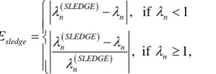
, if 1

, if 1, SLEDGE

n n n

SLEDGE sledge

n n

n SLEDGE

n

E

λ

 ₋ _<



=  ₋

≥ 



(6)

where (SLEDGE) n

λ

_{are the SLEDGE-squared eigenvalues and}λ_n_{are eigenvalues}

[image:16.595.300.457.74.128.2]

obtained by the SLEUTH and MG4 codes. This represents the absolute or rela-tive eigenvalue errors of each code relarela-tive to the benchmark values obtained from SLEDGE. The obtained absolute or relative eigenvalue errors of each code are used to measure the performance of each method. In Table 1, we see that the error characterization Esledge for the eigenvalues λ0, λ20 and λ100 obtained by the SLEUTH are slightly larger than the error characterization Esledge for the eigenvalues λ0, λ20 and λ100 achieved by the MG4 method.

Table 1. Eigenvalues of Problem 1.

Eval Index SLEDGE SLEUTH Esledge of SLEUTH MG4 Esledge of MG4

[image:16.595.60.539.287.347.2]

0 0.339260710091670 0.3392607100805489 1.105e−11 0.339260710092205 5.348e−13 20 73973.71134197622 73973.711342122158 1.973e−12 73973.711342028924 7.125e−13 100 39594796.88731044 39594796.886610150 1.769e−11 39594796.887332238 5.506e−13

[image:16.595.58.544.376.435.2]

0 236.0251207053473 236.02512061495375 3.830e−10 236.02512070536613 7.984e−14 50 3155257.7441797131 3155257.7441750434 1.480e−12 3155257.7441805508 2.655e−13 100 41735725.88393135 41735725.884191565 6.235e−12 41735725.883945607 3.415e−13

[image:16.595.52.539.467.527.2]

0 0.2786088184066070 0.2786088184207267 1.412e−11 0.27860881843425472 2.765e−11 50 6765204.5033669453 6765204.5033744955 1.116e−12 6765204.5033704005 5.107e−13 100 104060404.5008649 104060404.50095831 8.977e−13 104060404.50091156 4.485e−13

2 4871.3813098296687 4871.3813098537794 4.950e−12 4871.3813098332166 7.283e−13 50 7028539.5468045129 7028539.5468126526 1.158e−12 7028539.5467997193 6.820e−13 100 105083729.4441578 105083729.44410391 5.128e−13 105083729.44420157 4.166e−13

[image:16.595.55.543.559.618.2]

(17)

In Table 2, we see that the error characterization Esledge for the eigenvalues

0

λ , λ50 and λ100 obtained by the SLEUTH are slightly larger than the error characterization Esledge for the eigenvalues λ0, λ50 and λ100 achieved by the MG4 method. In Table 3, we see that the error characterization Esledge for the eigenvalues λ0 and λ100 achieved by the MG4 method are quite comparable to the error characterization Esledge for the eigenvalues λ0 and λ100 obtained by the SLEUTH. But, the error characterization Esledge for the eigenvalue λ50 obtained by the SLEUTH is slightly larger than the error characterization Esledge for the eigenvalue λ50 achieved by the MG4 method. In Table 4, we see that the error characterization Esledge for the eigenvalue λ100 achieved by the MG4 method is quite comparable to the error characterization Esledge for the eigen-value λ100 obtained by the SLEUTH. But, the error characterization Esledge for the eigenvalues λ2 and λ50 obtained by the SLEUTH are slightly larger than the error characterization Esledge for the eigenvalues λ2 and λ50 achieved by the MG4 method. In Table 5, we see that the error characterization Esledge for the eigenvalues λ0, λ8, λ30 and λ100 obtained by the SLEUTH are slightly larger than the error characterization Esledge for the eigenvalues λ0, λ8, λ30 and λ100 achieved by the MG4 method.

Remark 5.1 The machine precision, obtained from the FORTRAN routine EPSLON, on the desktop computer (with Pentium 4 processors) used to obtain the following outputs of the SLEUTH and SLEDGE codes was MACHEPS = 2.22D-16.

5. Conclusion

In this paper we have presented the MG4 algorithm of Iserles et al. [33] [40], for eigenvalue computation of regular 4th order Sturm-Liouville problems. Apply-ing the change to “Invariant-ImbeddApply-ing” variables in a manner similar to Green-berg and Marletta in their SLEUTH code [14] provides good stabilization for the MG4 algorithm, and this resulted in its capability for achieving high accuracy, very often on the order of machine precision. The MG4 algorithm appears to be competitive to the SLEUTH code.

Acknowledgements

The author would like to thank Al Baha University for their financial and moral support. The author would also like to express his sincere gratitude to the fol-lowing people:

1) Professor Charles Fulton and Dr. Steven Pruess for supplying a FORTRAN 90 version of the SLEDGE code.

2) Professor M. Marletta for supplying a FORTRAN 77 version of the SLEUTH code based on use of the BLAS underlying the LAPACK software, and for suggesting a modification to it which allowed us to run SLEUTH with high accuracy requests.

Conflicts of Interest

(18)

References

[1] Alalyani, A. (2019) Numerical Methods for Eigenvalue Computation of Fourth-Order Self-Adjoint Ordinary Differential Operators. PhD Dissertation, Florida Institute of Technology, Melbourne.

[2] Everitt, W.N. (1957) The Sturm-Liouville Problem for Fourth Order Differential Equations. The Quarterly Journal of Mathematics, 8, 146-160.

https://doi.org/10.1093/qmath/8.1.146

[3] Fulton, C. (1989) The Bessel-Squared Equation in the Lim-2, Lim-3, Im-4 Cases.

The Quarterly Journal of Mathematics, 40, 423-456.

https://doi.org/10.1093/qmath/40.4.423

[4] Bailey, P., Gordon, M. and Shampine, L. (1978) Automatic Solution of the Sturm- Liouville Problem. ACM Transactions on Mathematical Software, 4, 193-208.

https://doi.org/10.1145/355791.355792

[5] Bailey, P.B., Everitt, W.N. and Zettl, A. (2001) The SLEIGN2 Sturm-Liouville Code.

ACM Transactions on Mathematical Software, 21, 143-192.

https://doi.org/10.1145/383738.383739

[6] Pruess, S. and Fulton, C. (1993) Mathematical Software for Sturm-Liouville Prob-lems. ACM Transactions on Mathematical Software, 19, 360-376.

https://doi.org/10.1145/155743.155791

[7] Fulton, C. and Pruess, S. (1998) The Computation of Spectral Density Functions for Singular Sturm-Liouville Problems Involving Simple Continuous Spectra. ACM Transactions on Mathematical Software, 34, 107-129.

https://doi.org/10.1145/285861.285867

[8] Pryce, J.D. (1993) Numerical Solution of Sturm-Liouville Problems. Oxford Univer-sity Press, Oxford.

[9] Pryce, J.D. and Marletta, M. (1992) Automatic Solution of Sturm-Liouville Prob-lems Using the Pruess Method. Journal of Computational and Applied Mathemat-ics, 39, 57-78.https://doi.org/10.1016/0377-0427(92)90222-J

[10] Pryce, J. (1986) Error Control of Phase-Function Shooting Methods for Sturm-Liouville Problems. IMA Journal of Numerical Analysis, 6, 103-123.

https://doi.org/10.1093/imanum/6.1.103

[11] Ledoux, V., Van Daele, M. and Vanden Berghe, G. (2004) CP Methods of Higher Order for Sturm-Liouville and Schrödinger Equations. Computer Physics Commu-nications, 162, 153-165.https://doi.org/10.1016/j.cpc.2004.07.001

[12] Ledoux, V., Van Daele, M. and Vanden Berghe, G. (2005) MATSLISE: A Matlab Package for the Numerical Solution of Sturm-Liouville and Schrödinger Equations.

ACM Transactions on Mathematical Software, 31, 532-554.

https://doi.org/10.1145/1114268.1114273

[13] Ixaru, L. (2000) CP Methods for the Schrödinger Equation. Journal of Computa-tional and Applied Mathematics, 125, 347-357.

https://doi.org/10.1016/S0377-0427(00)00478-7

[14] Greenberg, L. and Marletta, M. (1997) Algorithm 775: The Code SLEUTH for Solv-ing Fourth-Order Sturm-Liouville Problems. ACM Transactions on Mathematical Software, 23, 453-493.https://doi.org/10.1145/279232.279231

(19)

DOI: 10.4236/am.2019.109056 802 Applied Mathematics [16] Greenberg, L. (1991) An Oscillation Method for Fourth-Order, Self-Adjoint, Two-Point Boundary Value Problems with Nonlinear Eigenvalues. SIAM Journal on Mathe-matical Analysis, 22, 1021-1042.https://doi.org/10.1137/0522067

[17] Chanane, B. (2010) Accurate Solutions of Fourth Order Sturm-Liouville Problems.

Journal of Computational and Applied Mathematics, 234, 3064-3071.

https://doi.org/10.1016/j.cam.2010.04.023

[18] Chanane, B. (1998) Eigenvalues of Fourth Order Sturm-Liouville Problems Using Fliess Series. Journal of Computational and Applied Mathematics, 96, 91-97.

https://doi.org/10.1016/S0377-0427(98)00086-7

[19] Chanane, B. (2002) Fliess Series Approach to the Computation of the Eigenvalues of Fourth-Order Sturm-Liouville Problems. Applied Mathematics Letters, 15, 459-563.

https://doi.org/10.1016/S0893-9659(01)00159-8

[20] Chanane, B. (1998) Eigenvalues of Sturm-Liouville Problems Using Fliess Series.

Applicable Analysis, 69, 233-238.https://doi.org/10.1080/00036819808840659 [21] Mihaila, B. and Mihaila, I. (2002) Numerical Approximations Using Chebyshev

Po-lynomial Expansions: El-gendi’s Method Revisited. Journal of Physics A: Mathe-matical and General, 35, 731-746.https://doi.org/10.1088/0305-4470/35/3/317 [22] El-Gamel, M. and Sameeh, M. (2012) An Efficient Technique for Finding the

Ei-genvalues of Fourth-Order Sturm-Liouville Problems. Applied Mathematics, 3, 920-925.https://doi.org/10.4236/am.2012.38137

[23] El-Gamel, M. and Abd El-hady, M. (2013) Two Very Accurate and Efficient Me-thods for Computing Eigenvalues of Sturm-Liouville Problems. Applied Mathemat-ical Modeling, 37, 5039-5046.https://doi.org/10.1016/j.apm.2012.10.019

[24] Fox, L. (1962) Chebyshev Methods for Ordinary Differential Equations. The Com-puter Journal, 4, 318-331.https://doi.org/10.1093/comjnl/4.4.318

[25] Saleh Taher, A.H., Malek, A. and Momeni-Masuleh, S.H. (2013) Chebyshev Diffe-rential Matrices for Efficient Computation of the Eigenvalues of Fourth-Order Sturm-Liouville Problems. Applied Mathematical Modeling, 37, 4634-4642.

https://doi.org/10.1016/j.apm.2012.09.062

[26] Ycel, U. (2015) Numerical Approximations of Sturm-Liouville Eigenvalues Using Chebyshev Polynomial Expansions Method. Cogent Mathematics, 2, Article ID: 1045223.https://doi.org/10.1080/23311835.2015.1045223

[27] Ycel, U. and Boubaker, K. (2012) Differential Quadrature Method (DQM) and Boubaker Polynomials Expansion Scheme (BPES) for Efficient Computation of the Eigenvalues of Fourth-Order Sturm-Liouville Problems. Applied Mathematical Modelling, 36, 158-167.https://doi.org/10.1016/j.apm.2011.05.030

[28] Khmelnytskaya, K., Kravchenko, V. and Baldenebro-Obeso, J. (2012) Spectral Pa-rameter Power Series for Fourth-Order Sturm-Liouville Problems. Applied Mathe-matics and Computation, 219, 3610-3524.

https://doi.org/10.1016/j.amc.2012.09.055

[29] Kravchenko, V. and Porter, R. (2010) Spectral Parameter Power Series for Sturm- Liouville Problems. Mathematical Methods in the Applied Sciences, 33, 459-468.

https://doi.org/10.1002/mma.1205

[30] Kravchenko, V. and Porter, R. (2015) Eigenvalue Problems, Spectral Parameter Power Series, and Modern Applications. Mathematical Methods in the Applied Sciences, 38, 1945-1969. https://doi.org/10.1002/mma.3213

(20)

Operators, Dundee, Lecture Notes in Mathematics 1032, 240-256.

https://doi.org/10.1007/BFb0076800

[32] Atkinson, F. (1964) Discrete and Continuous Boundary Problems. Academic Press, New York.https://doi.org/10.1063/1.3051875

[33] Iserles, A., Marthinsen, A. and Nrsett, S.P. (1999) On the Implementation of the Method of Magnus Series for Linear Differential Equations. BIT Numerical Mathe-matics, 39, 281-304.https://doi.org/10.1023/A:1022393913721

[34] Greenberg, L. and Marletta, M. (1997) The Validity of Richardson Extrapolation in Coefficient Approximation Methods for Fourth Order and Higher Order Self-Adjoint ODE Eigenvalue Problems. Technical Report, Department of Mathe-matics and Computer Science, University of Leicester, Leicester.

[35] Greenberg, L. (1991) A Prüfer Method for Calculating Eigenvalues of Self-Adjoint Systems of Ordinary Differential Equations: Parts 1 and 2. Technical Report TR91-24, University of Maryland at College Park, College Park.

[36] Gallier, J. (2005) Manifolds, Lie Groups, Lie Algebras, Riemannian Manifolds, with Applications to Computer Vision and Robotics [Lecture Notes]. Department of Computer and Information Science, University of Pennsylvania, ‎Philadelphia. [37] Magnus, W. (1954) On the Exponential Solution of Differential Equations for a

Li-near Operator. Communications on Pure and Applied Mathematics, 7, 649-673.

https://doi.org/10.1002/cpa.3160070404

[38] Iserles, A. and Nrsett, S.P. (1999) On the Solution of Linear Differential Equations in Lie Groups. Philosophical Transactions of the Royal Society A: Mathematical,

Physical and Engineering Sciences, 357, 983-1019.

https://doi.org/10.1098/rsta.1999.0362

[39] Stoer, J. and Bulirsch, R. (1993) Introduction to Numerical Analysis. Second Edi-tion, Springer-Verlag, New York.https://doi.org/10.1007/978-1-4757-2272-7 [40] Iserles, A., Munthe-Kaas, H.Z., Norsett, S.P. and Zanna, A. (2005) Lie-Group