Sexual selection and assortative mating: an experimental
1
test
2
ALLAN DEBELLE1, MICHAEL G. RITCHIE2AND RHONDA R. SNOOK3
3
1School of Life Sciences, University of Sussex, JMS Building, Brighton, BN1 9QG, UK
4
2School of Biology, University of St Andrews, Dyers Brae House, St Andrews, Fife, KY16 9TH, UK
5
3Animal and Plant Sciences, University of Sheffield, Alfred Denny Building, Sheffield, S10 2TN, UK 6
Correspondence: 7
A. Debelle 8
mailing address: JMS Building, University of Sussex, BN1 9QG Brighton, United Kingdom 9
e-mail address:[email protected]
10
phone number : +44 1273 877247 11
Running title: Sexual selection and assortative mating 12
Abstract
14
Mate choice and mate competition can both influence the evolution of sexual isolation 15
between populations. Assortative mating may arise if traits and preferences diverge in step, 16
and, alternatively, mate competition may counteract mating preferences and decrease 17
assortative mating. Here we examine potential assortative mating between populations of 18
Drosophila pseudoobscura that have experimentally evolved under either increased 19
(‘polyandry’) or decreased (‘monogamy’) sexual selection intensity for 100 generations. 20
These populations have evolved differences in numerous traits, including a male signal and 21
female preference traits. We use a 2 males: 1 female design, allowing both mate choice and 22
competition to influence mating outcomes, to test for assortative mating between our 23
populations. Mating latency shows subtle effects of male and female interactions, with 24
females from the monogamous populations appearing reluctant to mate with males from 25
the polyandrous populations. However, males from the polyandrous populations have a 26
significantly higher probability of mating regardless of the female’s population. Our results 27
suggest that if populations differ in the intensity of sexual selection, effects on mate 28
competition may overcome mate choice. 29
Keywords:Drosophila; experimental evolution; mate competition; female preference; sexual 30
conflict; sexual isolation; speciation. 31
Introduction
33
Sexual selection is often thought to be an important force in the origin of sexual isolation 34
between populations, although this is subject to much debate (Mayr, 1963; Coyne & Orr, 35
2004; Rundle & Nosil, 2005; Sobelet al.,2010; ITN Marie Curie Speciation, 2011). Intersexual 36
selection may facilitate sexual isolation because coevolution of mating signals and 37
associated preferences may lead to divergence between populations. This divergence would 38
then have the potential to generate assortative mating (i.e. a higher likelihood of mating 39
with an individual from the same population) if populations come into secondary contact 40
(Lande, 1981; Kirkpatrick, 1982; Price, 1998; Kirkpatrick & Ravigné, 2002; Uyedaet al.,2009). 41
While divergence in preferences between populations is often matched by signal divergence 42
(Rodríguez et al., 2013), strong preferences may theoretically decrease isolation if 43
preference genes introgress between species (Servedio & Bürger, 2014). Likewise, strong 44
sexual selection can influence mate competition, which may facilitate population 45
divergence, for example by reinforcing the action of mating preference on a given mating 46
signal. Strong mate competition may also constrain the expression of mating preferences by 47
reducing the opportunities to mate with preferred, but less competitive, mates (Wong & 48
Candolin, 2005; Hunt et al., 2009). Thus, it is difficult to predict the overall influence of 49
sexual selection on sexual isolation. 50
Experimental sexual selection directly manipulates a species’ mating system to observe, in 51
real time, the evolutionary consequences on sexual traits, mating patterns, and the 52
evolution of reproductive isolation (Holland & Rice, 1999; Martin & Hosken, 2003, 2004; 53
Wigby & Chapman, 2004, 2006; Crudgingtonet al.,2005, 2010; Rundle & Chenoweth, 2005; 54
experimental sexual selection in Drosophila pseudoobscura by either enforcing monogamy 56
(1 male:1 female) or promoting polyandry (1 female:6 males) and found a variety of 57
evolutionary responses. For example, divergence between monogamous and polyandrous 58
populations in an important male courtship signal has occurred, with males from 59
polyandrous populations singing a faster courtship song compared to males from 60
monogamous populations (Snook et al., 2005). There is also evidence for coevolution of 61
female preference for song; in playback experiments, females from the polyandrous 62
populations prefer polyandrous-like male song whereas females from monogamous 63
populations preferred monogamous-like song (Debelle et al., 2014). Other traits that are 64
implicated in sexual selection, such as cuticular hydrocarbon profiles, have also diverged 65
between the sexual selection treatments (Huntet al.,2012). 66
Here we conduct what is referred to as a “choice” experiment in which mating trials involve 67
2 males: 1 female (Dougherty & Shuker, 2014) from replicate polyandrous and monogamous 68
populations to examine how the evolutionary history of these populations influences mating 69
patterns. This type of design was chosen at it usually results in a stronger expression of 70
mating preferences compared to no-choice designs (Dougherty & Shuker, 2014). Moreover, 71
such a design allows mating patterns to be influenced by both male-male and male-female 72
interactions, and is considered to be the most appropriate way to test for sexual isolation 73
between populations (Coyneet al.,2005). 74
If female choice predominates mating interactions, we predict to observe a significant effect 75
of both male and female evolutionary history on mating patterns. These effects could 76
potentially result in assortative mating occuring within each replicate population of each 77
treatment (i.e. between-replicate) variation in patterns of song-preference divergence 79
between the sexual selection treatments (Debelle et al. 2014), suggesting that sexual 80
selection treatment consistently influences the direction of signal-preference coevolution in 81
our populations (and other traits that may have diverged between treatments). We thus 82
predict that if female choice predominates mating interactions, then assortative mating by 83
treatment will occur (i.e. polyandrous females with polyandrous males and monogamous 84
females with monogamous males). 85
Alternatively, male-male competition could largely predominate mating interactions, 86
resulting in finding no effect of female evolutionary history on mating patterns. Males from 87
polyandrous populations present a higher courtship frequency (Crudgington et al., 2010), a 88
trait that could be implicated in male-male competition (e.g. Shine et al. 2005; Kim and 89
Velando 2014). Additionally, male-male interactions are common between rival males of this 90
species placed in a choice design (e.g. chasing, courtship interruption, physical threats and 91
attacks; see Figure S1 in Appendix 1). We would therefore further predict that polyandrous 92
males, who continuously experience strong male-male competition, will win more matings 93
than monogamous males, regardless of female evolutionary history. 94
We test these alternative predictions by examining the mating patterns between the 95
experimental populations after 100 generations of experimental evolution. To standardise 96
female response against selection males, we also conduct the same experiment using 97
females from the ancestral population. Because these females do not discriminate between 98
male songs from the polyandrous and monogamous treatments (Debelle et al., 2014), we 99
expect to observe random mating patterns. However, if male-male competition influences 100
patterns as that of selection line females. We test for body size differences between our 102
populations and treatments, and include it as a covariate in our analyses, because body size 103
is frequently targeted by sexual selection and has a large influence on male mating success 104
(Blanckenhorn, 2000). In Drosophila species, larger males win more aggressive encounters 105
with other males (Partridge & Farquhar 1983; Partridgeet al.,1987a), deliver more courtship 106
(Partridge et al., 1987a,b) and mate faster (Partridge & Farquhar, 1983). We discuss how 107
sexual selection influences mating outcome and the implications of these results for 108
population divergence and speciation. 109
Material and Methods
110
Sexual selection treatments
111
The selection lines are described in detail in Crudgington et al.,(2005). Briefly, an ancestral 112
wild-caught population of the naturally polyandrous speciesDrosophila pseudoobscurafrom 113
Tucson (Arizona, USA) was used to establish the selection lines. Four replicate populations 114
(replicate 1, 2, 3 and 4) of two different sexual selection treatments were established. Adult 115
sex-ratio in vials is manipulated by either confining one female with a single male 116
(‘monogamy’ treatment; M) or one female with 6 males (‘elevated polyandry’ treatment;E) 117
in vials. Henceforth, reference to E or M refers to the experimental sexual selection 118
treatment flies derive from. Effective population sizes are equalized between the treatments 119
(Snook et al., 2009). At each generation, offspring are collected and pooled together for 120
each replicate population, and a random sample used to constitute the next generation in 121
the appropriate sex-ratios, thus proportionally reflecting the differential offspring 122
maintained, in standard food vials (2.5mm x 80mm) and with a generation time of 28 days. 124
The ancestral population (A) is also maintained, in bottles (57 mm x 132 mm) with an equal 125
sex-ratio of adult flies. All populations are kept at 22oC on a 12L:12D cycle, with standard
126
food media and added live yeast. 127
Experimental flies
128
To generate the experimental flies, 50 reproductively mature adults (25 males and 25 129
females) of each treatment (E and M) and replicate (1, 2, 3 and 4) were used as parents and 130
kept in mass-cultures, providing a common social context for parents of both sexual 131
selection treatments. The resulting larvae were raised in controlled density vials (100 first 132
instar larvae per food vial). Flies from these vials were collected and sexed on the day of 133
hatching using CO2 anaesthetization. Virgin males and females were kept separate in
134
yeasted food vials with a maximum of 20 individuals per vial, and used in mating 135
experiments once they had reached sexual maturity (four to six days old; Snook & Markow, 136
2001). Experimental females from the ancestral population were also generated using the 137
same method. 138
To identify the population of origin of males, we clipped a small corner off the right lower 139
wing margin of half of the males, under CO2 anaesthetization, two days before the
140
experiment. Wing clipping has no effect on male mating success in D. pseudoobscura (e.g. 141
Dodd, 1989) but, as a control, half the males from each treatment were clipped. The males 142
were then stored in vials of 12 individuals of the same population until the experiment. 143
Assortative mating design
We tested for assortative mating between the different populations by placing one female (E 145
or M) in a food vial with two males (one E and one M). Competing males always came from 146
the same replicate (e.g., one E1 and one M1 male, or one E3 and one M3 male). All the 147
female-male combinations between populations were tested: we crossed the 8 female 148
populations (E1-4; M1-4) with the 4 possible pairs of males (E1 and M1; E2 and M2; E3 and 149
M3; E4 and M4), for a total of 32 combinations. For each combination, the minimum sample 150
size was 40 females (N=1280 trials in total). Reproductively mature males were loaded first 151
into food vials, followed by reproductively mature females, and each vial was observed until 152
mating occurred, or for 20 minutes. If mating occurred, then the identity of the mating male 153
was recorded (E or M). If no mating occurred, then the trial was discarded (N=116 trials). 154
Both mating latency and mating outcome (i.e. the identity of the winning male: E or M) were 155
measured. Mating latency, defined here as the time between introducing the female into 156
the vial until the start of mating, is an important component ofDrosophilamale competitive 157
success and female preference (e.g. Bacigalupe et al.,2007). Mating outcome was used to 158
predict the probability of an E or an M male winning with the different female populations. 159
The same design was used with females from the ancestral (A) population (one A female 160
with one E and one M male). 161
To examine a potential role of body size on mating patterns in our experiment, the length of 162
wing vein IV of each individual (male and female) was measured as an estimate of body size 163
(Crudgingtonet al.,2005) and included in the statistical analyses. Wings were mounted in a 164
30% glycerol-70% ethanol medium, photographs taken using a Motic camera and Motic 165
Images Plus 2.0 software (Motic Asia, Hong Kong), and wing vein length measured with 166
courtship behaviors (O’Dell, 2003), we measured temperature during trials using a Testo 168
735-1 thermometer (Testo Limited, United Kingdom), and subsequently used temperature 169
as a covariate in the analyses (mean temperature during the time of each trial). The 170
experiment was performed in 2-hour sessions, when the incubator lights came on, to mimic 171
the D. pseudoobscura activity pattern (Noor, 1998). The different crosses were randomly 172
assigned across the different days. The generations of the sexual selection treatments used 173
were: replicate 1= 102, 105 and 107; replicate 2= 101, 104 and 106; replicate 3= 100, 103 174
and 105; replicate 4= 98, 101 and 103. The generation of the ancestral population used was 175
124. 176
Predictions and statistical analyses
177
Our main objective was to distinguish between three alternative outcomes: assortative 178
mating could occur between replicate populations (i.e. a polyandrous male is more likely to 179
mate with a polyandrous female from its own replicate population), or between sexual 180
selection treatments (i.e. a polyandrous male is more likely to mate with a polyandrous 181
female regardless of their respective replicate population), or not occur at all (i.e. matings 182
could be mostly won by polyandrous males). We expect the non-coevolved ancestral 183
females to mate randomly, given that at least for song, they exhibit no distinct preference. 184
However this population is also subject to sexual selection, so predicting mating outcome is 185
more difficult than in the polyandrous and monogamous populations. Thus, results of 186
mating patterns for the females from the ancestral population were analysed separately. 187
Mating latency is used to measure female preference in Drosophila, with shorter latencies 188
al., 2014). A simple prediction then would be that mating outcome patterns are reflected in 190
the mating latency patterns. However, this prediction is complicated by the potential action 191
of sexual conflict, that could lead to polyandrous (and/or bigger) females exhibiting more 192
resistance to mating, thereby increasing mating latency (Arnqvist & Rowe, 2005), and male-193
male competition, that could also affect mating latency(Bretmanet al., 2009). 194
To test these predictions, we scored the winners of the mating encounters and measured 195
mating latency. For both mating outcome and latency, we also included ‘type of cross’ in the 196
model to test whether populations experiencing sexual conflict/sexual selection show 197
greater measures of sexual isolation (for review, see Gavrilets, 2014). The crosses involving a 198
male from the same population as the female (i.e. “coevolved”; e.g., an E1 female with an E1 199
and a M1 male or M1 female with an E1 and a M1 male) were considered as ’within 200
population’ crosses and all the other combinations were ’between populations’ crosses (e.g., 201
an E1 female with an E2 and a M2 male). The category ’within population’ was further 202
divided into two subcategories, ‘within E population’ when the E male and the E female were 203
from the same population (e.g., E1 female, E1 male, M1 male) and ‘within M population’ 204
when the M male and the M female were from the same population (e.g., M2 female, M2 205
male, E2 male). 206
To examine any effect of male and female body size on male mating success, we first tested 207
for differences in absolute body size of males and females between the sexual selection 208
treatments. These were tested both within replicate (e.g., E1 males vs. M1 males, or E3 209
females vs. M3 females) and with all replicates combined (E males vs. M males, and E 210
females vs. M females), using Wilcoxon rank sum tests as size was not normally distributed. 211
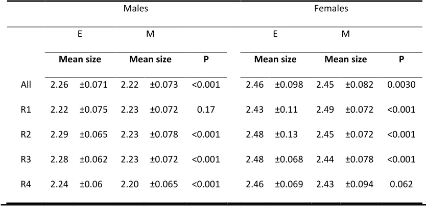
Average body size differed significantly between the treatments, with both E males and 213
females being overall larger than their M counterparts, either taking all replicates into 214
account or across most replicates (Table 1). To disentangle the effect of body size on mating 215
patterns from the action of other traits that responded to sexual selection manipulation, we 216
ran statistical models analysing both mating outcome and latency either with absolute male 217
and female body size as covariates (presented within the text) or without (Appendix S1). 218
We analysed mating outcome (whether E or M males win) using a generalized linear mixed 219
model with a binomial distribution. We specifically investigated what variables influence the 220
probability of the two possible mating events (‘E male wins’ versus ‘M male wins’; ‘E male 221
wins’ was used as the reference event). Female treatment, male replicate, E and M male 222
size, E and M male relative size difference, female size, the temperature and the type of 223
cross were included as fixed effects in the model. The interaction between female treatment 224
and male replicate was also tested. Male and female replicate were nested within their 225
respective sexual selection treatment. This analysis models the probability of an E male 226
winning. We ran the same model for A females, with the exception that ‘female treatment’, 227
‘type of cross’, and ‘female replicate’ were obviously not included as effects in the model. 228
To test the mating latency response, we first log-transformed mating latency and then 229
analysed it using a linear mixed model with a Gaussian distribution. Female treatment (‘E’ 230
was used as the reference level), winning male treatment (‘E’ was used as the reference 231
level), absolute body sizes of both males and of the female, temperature and type of cross 232
(‘between populations’ was used as the reference level) were included as fixed effects. In 233
addition to absolute male and female body sizes, the relative body size difference between 234
levels: ‘E larger than M’ or ‘E smaller than M’ than M; ‘E smaller than M’ was used as the 236
reference level). The interactions between winning male and female treatment (to test for 237
assortative mating within sexual selection treatment), and between type of cross and 238
winning male treatment (to test for a difference between the treatments in assortative 239
mating within population), were also tested. Male and female replicate were nested within 240
their respective sexual selection treatment, to account for variation among the replicated 241
populations (Garland & Rose, 2009). This analysis models the speed it takes males from the 242
different selection lines to mate with females of the different selection lines. We ran the 243
same model for A females, with the exception that ‘female treatment’ and ‘type of cross’ 244
could not be included as main effects and ‘female replicate’ could not be included as a 245
random effect in the model. 246
In all the mixed models described above, the significance of fixed effects was tested using 247
likelihood ratio tests. Normality and homoscedasticity of the residuals were checked 248
graphically. Model estimates were used in figures, adjusted for the effects of all the other 249
variables not included in the figure. All statistical analyses were performed in R (R 250
Development Core Team 2005). The lme4 library was used for mixed-models (Bates & 251
Sarkar, 2007), and theglht function in themultcomplibrary was used for post-hoc analysis 252
of the mixed-model results (Hothornet al., 2008). Raw mating outcome and mating latency 253
data are also shown in Appendix S1 (see Fig. S2 and S3). 254
Results
255
There is no effect of the type of cross (that is, whether the female and the mating male are 256
M males are faster to mate or more likely to mate when they are in the presence of a female 258
from their own population (Table 2). Instead, E males win significantly more matings with all 259
females and mate overall at least as quickly as M males. 260
In the case of mating outcome, E males win more matings than M males regardless of 261
female treatment (for E females: E males = 377, M males = 146, = 98.83, P<0.001 ; for M 262
females : E males = 360, M males = 136, = 101.16, P<0.001). The mixed-model approach 263
confirms this pattern, finding a much higher mating success of E males in comparison to M 264
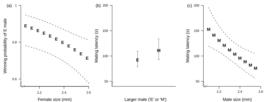
males (i.e., E males have a mating probability greater than 0.5 regardless of their replicate 265
population; Fig. 1a; Table 2), and no significant effect of female treatment on the mating 266
outcome (Table 2). Neither the relative size difference between the males, nor male 267
absolute body sizes, have a significant effect on mating outcome (Table 2), meaning that the 268
higher mating probability of E males is not the result of their larger size. In contrast to males, 269
female size significantly influences the probability of an E male winning: E males are less 270
successful with larger females (Table 2; Fig. 2a). Running the model without male and female 271
body size shows the same pattern of treatment effect on mating outcome (see Table S1 of 272
Appendix S1). 273
For mating latency, there is a significant interaction between winning male treatment and 274
female treatment (Fig. 1b; Table 2). E females mate faster with E males when E males win, 275
and mate slower with M males when M males win. In contrast, M females mate as quickly 276
with M males as they do with E males. That is, when M males win, it takes them longer to 277
effect on mating latency. The relative size difference between the E and the M male 279
influences mating latency, with mating latency being shorter when the E male is larger than 280
the M male (Fig. 2b ; Table 2). M male absolute size is negatively associated with mating 281
latency; that is, as M male size increases, males start mating with females earlier (Fig. 2c ; 282
Table 2). Overall, these results suggest that larger males, particularly M males, start mating 283
earlier than smaller males. In contrast, female size has no significant effect on mating 284
latency (Table 2). Running the model without male and female body size shows the same 285
direction of treatment effects on mating latency (see Table S1 of Appendix S1). 286
Mating trials with ancestral females show that E males also have a higher probability of 287
winning matings than M males (Fig. 3a; Table 3) and that M males take longer than E males 288
to achieve matings with ancestral females (Fig. 3b; Table 3). Ancestral female body size have 289
no effect on mating outcome or latency, likely because these females exhibit less variation in 290
body size than selection lines females (Levene’s test: F1=39.57, P<0.001). Running models
291
without body size shows the same pattern of treatment effects (see Table S2 of Appendix 292
S1). 293
Discussion
294
We used an experimental approach to understand how changes in sexual selection intensity 295
can influence assortative mating in a system in which we have quantified changes in traits 296
related to both intra- and inter- sexual selection. We find that assortative mating is not 297
observed, either between treatments, or within sexual selection treatments. Instead, males 298
higher mating success, winning about 4 times more often than M males, regardless of 300
female selection history. 301
What might cause these mating patterns? Predictions of assortative mating largely derive 302
from an expectation of greater male-female coevolution under strong sexual selection 303
(Lande, 1981; Kirkpatrick, 1982; Price, 1998; Kirkpatrick & Ravigné, 2002; Uyedaet al.,2009). 304
There is evidence in our populations for coevolved song and female song preferences 305
(Debelleet al.,2014) which may generate assortative mating. Song in this species is used as 306
a species-specific signal, suggesting it is important in determining mating success and in 307
reproductive isolation (Williams et al., 2001). We have measured a variety of other male 308
traits in these populations that are thought to potentially influence pre-mating sexual 309
selection and found divergent responses between the treatments in some (cuticular 310
hydrocarbon profiles; courtship frequency; Hunt et al., 2012; Crudgington et al., 2010) but 311
not all (sex comb tooth number; Snook et al., 2013) traits. The extent to which female 312
preferences has changed for non-song traits have not been measured. 313
However, because we find that E males equally win with all types of females, it seems 314
unlikely that male-female coevolution can explain our patterns of mating success. Yet, this 315
does not mean that coevolution between the sexes has not occurred. Patterns of mating 316
latency may provide some evidence of coevolution. Most interestingly, while E males mate 317
faster than M males with females from populations experiencing polyandry (E and A), this 318
difference is not seen with M females. When M males do win matings with M females, this is 319
achieved faster than when M males win matings with E females. Therefore M males do seem 320
to benefit from a relative mating advantage with M, and only M, females. This advantage 321
2014). However, E males mate as fast as M males with M females, implying that E males can 323
override this female preference. 324
Varying the intensity of sexual selection will also have targeted traits that evolve under 325
male-male competition. Mate competition can override female mating preference by 326
reducing the ability of females from detecting, evaluating and/or mating with preferred 327
mates (Wong & Candolin, 2005), for example by intensifying courtship (i.e. decreasing 328
courtship latency or increasing courtship rate) to maximise their mating success. Courtship 329
rate commonly increases in a competitive context, as shown in sticklebacks (Shine et al., 330
2005), garter snakes (Kim & Velando, 2014) or fiddler crabs (Milner, 2012). Other 331
experimental evolution studies have found that males from monogamous populations 332
evolve reduced competitive mating success (Kawecki et al., 2012). The fact that E males 333
initiate courtship faster and court more frequently than M males (Snook et al., 2005; 334
Crudgington et al., 2010) may then influence the ability of females to detect and evaluate 335
between males (Shaw & Lugo, 2001). Another trait potentially associated with competitive 336
mating success is body size (Blanckenhorn, 2000). We found that the relative size difference 337
between the E and the M male influenced mating latency, such that mating latency was 338
shorter when the E male was larger than the M male. Larger M males also experienced a 339
mating benefit; we found that as M male size increased, mating latency decreased. 340
Generally then larger body size, particularly of E males, may influence mating patterns. This 341
result has been shown in other Drosophila species where larger males mate faster due to 342
their increased locomotor activity (Partridgeet al.,1987b; Long & Rice, 2007).
343
While male body size was important in determining mating latency, neither absolute male 344
of male body size in mediating mating success in D. pseudoobscura is unclear; in some 346
studies, larger males are more likely to be paired with females than smaller males (Partridge 347
et al.,1987a) but in other studies this body size advantage was not observed (Markow, 1988; 348
Markow & Ricker, 1992). Instead of a male effect, we found that female body size had an 349
influence on what male won, with E males being more likely to win with smaller compared 350
to larger females. This suggests sexual conflict over mating decisions (Clutton-Brock & 351
Parker, 1995). Sexual conflict occurs in our polyandrous populations and is eliminated in our 352
monogamous populations (Crudgington et al., 2005, 2010). Increased male mating 353
persistence can evolve under sexual conflict (Arnqvist & Rowe, 2005) and E males are more 354
persistent than M males (Crudgingtonet al.,2010). Smaller, less resistant M females, may be 355
less able to resist such males. We did not observe an overall effect of female treatment on 356
mating latency or outcome, but the mating latency and size effects on mating success 357
described here suggest that subtle interactions influence the outcome of the mating trials. 358
Male-male competition and female preference are not mutually exclusive forms of selection. 359
For example, rapid, vigorous courtship may be selected for when mate competition is high, 360
but will also be indirectly targeted by female preferences. Females are likely to obtain 361
indirect benefits from mating with males who can out-compete other males. In this sense 362
separating sources of selection into intra- versus intersexual selection is simplistic. However, 363
the fact that we see polyandrous males succeeding in mating trials, despite some evidence 364
for coevolution between the sexes in the experiment, suggests that greater selection on 365
male competitive courtship ability in the polyandrous populations has overwhelmed any 366
selection likely to cause assortative mating between populations from the treatments (or 367
suggested that if sexual conflict over mating outcome was strong, competitive males could 369
act as a force for gene flow and inhibit speciation (alternatively, if female choice 370
predominates, sexual conflict could increase speciation by assortative mating). Our results 371
are more compatible with the “males ahead” outcome of this model, with polyandrous 372
males, evolving under strong sexual selection, winning out in mating competitions with 373
males and females from different evolutionary histories. Overall, this suggests that sexual 374
selection has the potential to inhibit, as well as to increase, assortative mating and 375
speciation (Servedio, 2004). 376
Acknowledgements
377
We are grateful to undergraduate students Hugh Smith, Hanna Bennett, and David John, and 378
to lab members Helen Crudgington, Jessica Edwards, Sarah Fahle, Sarah Fellows and Nelly 379
Gidaszewski for their assistance with data collection, and to Alexandre Courtiol for 380
discussions about statistical analyses. This work was funded by the Marie Curie Initial 381
Training Network ‘Understanding the evolutionary origin of biological diversity’ (ITN-2008-382
213780 SPECIATION), and by a US National Science Foundation grant (DEB 0093149) and 383
NERC grants (NE/B504065/1; NE/D003741/1) to RRS. We thank all the participants of this 384
network for fruitful comments and discussions about this project, and particularly Anneli 385
Hoikkala for her helpful insight throughout the project. 386
References
Abramoff, M.D., Magalhães, P.J. & Ram, S.J. 2004. Image processing with ImageJ. 388
Biophotonics Int.11: 36–42. 389
Arnqvist, G. & Rowe, L. 2005.Sexual conflict. Princeton University Press. 390
Bacigalupe, L.D., Crudgington, H.S., Hunter, F., Moore, A.J. & Snook, R.R. 2007. Sexual 391
conflict does not drive reproductive isolation in experimental populations ofDrosophila 392
pseudoobscura.J. Evol. Biol.20: 1763–1771. 393
Bacigalupe, L.D., Crudgington, H.S., Slate, J., Moore, A.J. & Snook, R.R. 2008. Sexual selection 394
and interacting phenotypes in experimental evolution: a study ofDrosophila 395
pseudoobscuramating behavior.Evolution.62: 1804–1812. 396
Bates, D. & Sarkar, D. 2007.lme4: Linear mixed-effects models using S4 classes. 397
Blanckenhorn, W.U. 2000. The evolution of body size: what keeps organisms small?Q. Rev. 398
Biol.75: 385–407. 399
Bretman, A., Fricke, C. & Chapman, T. 2009. Plastic responses of male Drosophila 400
melanogaster to the level of sperm competition increase male reproductive fitness. 401
Proc. R. Soc. B Biol. Sci.1705–1711. 402
Clutton-Brock, T. & Parker, G. 1995. Sexual coercion in animal societies.Anim. Behav.49: 403
1345–1365. 404
Coyne, J.A., Elwyn, S. & Rolán-Alvarez, E. 2005. Impact of experimental design onDrosophila 405
sexual isolation studies: direct effects and comparison to field hybridization data. 406
Coyne, J.A. & Orr, H.A. 2004.Speciation. Sinauer Associates Sunderland, MA. 408
Crudgington, H., Fellows, S. & Snook, R.R. 2010. Increased opportunity for sexual conflict 409
promotes harmful males with elevated courtship frequencies.J. Evol. Biol.23: 440–446. 410
Crudgington, H.S., Beckerman, A.P., Brüstle, L., Green, K. & Snook, R.R. 2005. Experimental 411
removal and elevation of sexual selection: does sexual selection generate manipulative 412
males and resistant females?Am. Nat.165: S72–87. 413
Debelle, A., Ritchie, M. & Snook, R.R. 2014. Evolution of divergent female mating preference 414
in response to experimental sexual selection.Evolution.68: 2524–2533. 415
Dodd, D. 1989. Reproductive isolation as a consequence of adaptive divergence in 416
Drosophila pseudoobscura.Evolution.43: 1308–1311. 417
Dougherty, L.R. & Shuker, D.M. 2014. The effect of experimental design on the 418
measurement of mate choice: a meta-analysis.Behav. Ecol.26: 311–319. 419
Garland, T. & Rose, M.R. 2009.Experimental evolution: concepts, methods, and applications 420
of selection experiments. University of California Press. 421
Gavrilets, S. 2014. Is Sexual Conflict an “ Engine of Speciation ”?Cold Spring Harb. Perspect. 422
Biol.6: a017723. 423
Holland, B. & Rice, W.R. 1999. Experimental removal of sexual selection reverses intersexual 424
antagonistic coevolution and removes a reproductive load.Proc. Natl. Acad. Sci. USA 425
Holm, S. 2012. Multiple confidence sets based on stagewise tests.J. Am. Stat. Assoc.94: 427
489–495. 428
Hothorn, T., Bretz, F. & Westfall, P. 2008. Simultaneous inference in general parametric 429
models.Biometrical J.50: 346–63. 430
Hunt, J., Breuker, C.J., Sadowski, J.A. & Moore, A.J. 2009. Male-male competition, female 431
mate choice and their interaction: determining total sexual selection.J. Evol. Biol.22: 432
13–26. 433
Hunt, J., Snook, R.R., Mitchell, C., Crudgington, H.S. & Moore, A.J. 2012. Sexual selection and 434
experimental evolution of chemical signals inDrosophila pseudoobscura.J. Evol. Biol. 435
25: 2232–41. 436
ITN Marie Curie Speciation. 2011. What do we need to know about speciation?TREE27: 27– 437
39. 438
Kawecki, T.J., Lenski, R.E., Ebert, D., Hollis, B., Olivieri, I. & Whitlock, M.C. 2012. Experimental 439
evolution.TREE27: 547–60. 440
Kim, S. & Velando, A. 2014. Stickleback males increase red coloration and courtship 441
behaviours in the presence of a competitive rival.Ethology120: 502–510. 442
Kirkpatrick, M. 1982. Sexual selection and the evolution of female choice.Evolution.36: 1– 443
12. 444
Kirkpatrick, M. & Ravigné, V. 2002. Speciation by natural and sexual selection: models and 445
Lande, R. 1981. Models of speciation by sexual selection on polygenic traits.Proc. Natl. Acad. 447
Sci. USA.78: 3721–3725. 448
Long, T. A. F. & Rice, W.R. 2007. Adult locomotory activity mediates intralocus sexual conflict 449
in a laboratory-adapted population ofDrosophila melanogaster.Proc. Biol. Sci.274: 450
3105–12. 451
Markow, T. A. 1988. Reproductive behavior ofDrosophila melanogasterandD. 452
nigrospiraculain the field and in the laboratory.J. Comp. Psychol.102: 169–173. 453
Markow, T. A. & Ricker, J.P. 1992. Male size, developmental stability, and mating success in 454
natural populations of threeDrosophilaspecies.Heredity.69: 122–7. 455
Martin, O. Y. & Hosken, D. 2004. Reproductive consequences of population divergence 456
through sexual conflict.Curr. Biol.14: 906–910. 457
Martin, O.Y. & Hosken, D.J. 2003. The evolution of reproductive isolation through sexual 458
conflict.Nature423: 979–982. 459
Mayr, E. 1963.Animal species and evolution.Harvard University Press. 460
Milner, R. 2012. Keeping up appearances: male fiddler crabs wave faster in a crowd.Biol. 461
Lett.8: 176–8. 462
Noor, M.A.F. 1998. Diurnal activity patterns ofDrosophila subobscuraandD. pseudoobscura 463
O’Dell, K.M.C. 2003. The voyeurs’ guide toDrosophila melanogastercourtship.Behav. 465
Processes64: 211–223. 466
Parker, G.A. & Partridge, L. 1998. Sexual conflict and speciation.Philos. Trans. R. Soc. 467
London. Ser. B Biol. Sci.353: 261–274. 468
Partridge, L., Ewing, A. & Chandler, A. 1987b. Male size and mating success inDrosophila 469
melanogaster : the roles of male and female behaviour. Anim. Behav.35: 555–562. 470
Partridge, L. & Farquhar, M. 1983. Lifetime mating success of male fruitflies (Drosophila 471
melanogaster) is related to their size.Anim. Behav.31: 871–877. 472
Partridge, L., Hoffmann, A. & Jones, J.S. 1987a. Male size and mating success inDrosophila 473
melanogasterandD. pseudoobscuraunder field conditions.Anim. Behav.35: 468–476. 474
Price, T. 1998. Sexual selection and natural selection in bird speciation.Philos. Trans. R. Soc. 475
B Biol. Sci.353: 251–260. 476
R Development Core Team. 2005. R: A language and environment for statistical computing. 477
Rodríguez, R.L., Boughman, J.W., Gray, D.A., Hebets, E.A., Höbel, G. & Symes, L.B. 2013. 478
Diversification under sexual selection: the relative roles of mate preference strength 479
and the degree of divergence in mate preferences.Ecol. Lett.16: 964–74. 480
Rundle, H., Chenoweth, S. & Blows, M. 2006. The roles of natural and sexual selection during 481
Rundle, H.D. & Chenoweth, S.F. 2005. Divergent selection and the evolution of signal traits 483
and mating preferences.PLoS Biol.3: 1988–1995. 484
Rundle, H.D. & Nosil, P. 2005. Ecological speciation.Ecol. Lett.8: 336–352. 485
Servedio, M.R. 2004. The what and why of research on reinforcement.PLoS Biol.2: 2032– 486
2035. 487
Servedio, M.R. & Bürger, R. 2014. The counterintuitive role of sexual selection in species 488
maintenance and speciation.Proc. Natl. Acad. Sci. USA111: 8113–8. 489
Shaw, K.L. & Lugo, E. 2001. Mating asymmetry and the direction of evolution in the Hawaiian 490
cricket genusLaupala.Mol. Ecol.10: 751–9. 491
Shine, R., Langkilde, T., Wall, M. & Mason, R. 2005. Alternative male mating tactics in garter 492
snakes, Thamnophis sirtalis parietalis.Anim. Behav.70: 387–396. 493
Snook, R., Robertson, A., Crudgington, H. & Ritchie, M. 2005. Experimental manipulation of 494
sexual selection and the evolution of courtship song inDrosophila pseudoobscura. 495
Behav. Genet.35: 245–255. 496
Snook, R.R., Brüstle, L. & Slate, J. 2009. A test and review of the role of effective population 497
size on experimental sexual selection patterns.Evolution.63: 1923–33. 498
Snook, R.R., Gidaszewski, N.A., Chapman, T. & Leigh, W. 2013. Sexual selection and the 499
evolution of secondary sexual traits : sex comb evolution in Drosophila.J. Evol. Biol.26:
500
Snook, R.R. & Markow, T.A. 2001. Mating system evolution in sperm-heteromorphic 502
Drosophila.J. Insect Physiol.47: 957–964. 503
Sobel, J.M., Chen, G.F., Watt, L.R. & Schemske, D.W. 2010. The biology of speciation. 504
Evolution.64: 295–315. 505
Uyeda, J.C., Arnold, S.J., Hohenlohe, P. a & Mead, L.S. 2009. Drift promotes speciation by 506
sexual selection.Evolution.63: 583–94. 507
Wigby, S. & Chapman, T. 2004. Female resistance to male harm evolves in response to 508
manipulation of sexual conflict.Evolution.58: 1028–1037. 509
Wigby, S. & Chapman, T. 2006. No evidence that experimental manipulation of sexual 510
conflict drives premating reproductive isolation inDrosophila melanogaster.J. Evol. 511
Biol.19: 1033–1039. 512
Williams, M.A., Blouin, A.G. & Noor, M.A.F. 2001. Courtship songs of Drosophila 513
pseudoobscura and D. persimilis. II. Genetics of species differences. Heredity. 86: 68– 514
77. 515
Wong, B.B.M. & Candolin, U. 2005. How is female mate choice affected by male 516
competition?Biol. Rev. Camb. Philos. Soc.80: 559–571. 517
Tables
[image:26.595.64.481.296.499.2]519
Table 1Average body size values (in millimetres) between the sexual selection treatment, by
520
sex and replicate. Standard deviation is given next to each average body size value. Wilcoxon 521
rank sum tests were performed between E and M treatments for all replicates combined, 522
and for each replicate, to compare body size differences between the sexual selection 523
treatments. P is the p-value. The sample size is N = 1019. E = polyandry, M = monogamy, R = 524
replicate. 525
Males Females
E M E M
Mean size Mean size P Mean size Mean size P
All 2.26 ±0.071 2.22 ±0.073 <0.001 2.46 ±0.098 2.45 ±0.082 0.0030
R1 2.22 ±0.075 2.23 ±0.072 0.17 2.43 ±0.11 2.49 ±0.072 <0.001
R2 2.29 ±0.065 2.23 ±0.078 <0.001 2.48 ±0.13 2.45 ±0.072 <0.001
R3 2.28 ±0.062 2.23 ±0.072 <0.001 2.48 ±0.068 2.44 ±0.078 <0.001
R4 2.24 ±0.06 2.20 ±0.065 <0.001 2.46 ±0.069 2.43 ±0.094 0.062
Table 2 Output of the mixed-model for mating outcome and mating latency analyses for 527
selection line females, including model estimates and tests statistics. In the mating outcome 528
model, the response variable was the probability of an E male winning the mating. In the 529
mating latency model, the response variable was the mating latency of the winning male. 530
Winner treatment is the sexual selection treatment of the winning male (E or M), female 531
treatment is the sexual selection treatment of the female (E or M), type of cross 532
distinguishes between ‘within E population’, ‘within M population’ and ‘between 533
populations’ crosses, and E-M relative size difference is the relative size difference between 534
the males (‘E larger’ or ‘E smaller’). The following elements are specified: the model 535
estimate(s) of each variable (β), the likelihood ratio statistic used to test the main effect of
536
each variable (LR) and the p-value of the likelihood ratio test (p). The sample size is N = 1019. 537
MATING OUTCOME MATING LATENCY
Fixed effects Factor level Parameters Parameters
β LR P β LR P
Winner treatment (WT) M - - - 0.30 16.2 0.0028
Female treatment (FT) M 0.047 0.1 0.79 0.13 5.8 0.055
Type of cross (TC)
within E 0.049
0.9 0.64
0.13
5.6 0.23
within M -0.22 -0.15
E male body size - -0.26 0.0 0.85 -0.10 0.04 0.85
M male body size - 0.74 0.3 0.80 -1.55 10.3 0.0013
E-M relative size difference E > M 0.055 0.002 0.97 0.18 4.9 0.027
Female body size - 2.33 7.5 0.0062 -0.44 1.8 0.17
Temperature - 0.035 1.5 0.21 -0.0088 0.7 0.39
WT * FT M winner and M female
--
--0.33 5.8 0.016
-WT * TC
M winner and within E - - - 0.075
1.6 0.44
M winner and within M - - - 0.25
Global intercept -8.56 9.48
Random effects variance
female replicate 0.010 0.012
male replicate 0.064 0.00087
Table 3Output of the mixed-model for mating outcome and mating latency analyses for ancestral females, including model estimates and tests 540
statistics. In the mating outcome model, the response variable was the probability of an E male winning the mating with an ancestral female. In 541
the mating latency model, the response variable was the mating latency of the winning male. Winner treatment is the sexual selection 542
treatment of the winning male (E or M) and E-M relative size difference is the relative size difference between the males (‘E larger’ or ‘E 543
smaller’). The following elements are specified: the model estimate(s) of each variable (β), the likelihood ratio statistic used to test the main
544
effect of each variable (LR) and the p-value of the likelihood ratio test (p). The sample size is N = 179. E = polyandry, M = monogamy. 545
MATING OUTCOME MATING LATENCY
Fixed effects Factor level Parameters Parameters
β LR P β LR P
Winner treatment (WT) M - - - 0.39 6.1 0.014
E male body size - -4.32 0.7 0.42 -0.022 0.0001 0.99
M male body size - -1.69 0.1 0.72 -1.22 0.5 0.49
E-M relative size difference E > M -0.49 0.5 0.46 0.20 0.6 0.42
Female body size - 3.38 0.7 0.39 0.83 0.3 0.58
Global intercept 7.91 -0.62
Random effect variance male replicate 0.43 <0.001
Figures
547
Fig. 1 Mating outcome probability and mating latency of selection line females. (a) Mating
548
outcome (probability of an E male winning). The letters represent the fitted mating 549
probabilities estimated by the mixed-model of an E male winning depending on female 550
sexual selection treatment (labels of the x-axis). As these probabilities are superior to 0.5, 551
the figure shows that E males have overall a higher mating success than M males. (b) Mating 552
latency depending on male and female sexual selection treatment. The letters represent the 553
fitted mating latencies estimated by the mixed-model of a male winning depending on male 554
sexual selection treatment (the plotted values) and female sexual selection treatment (labels 555
of the x-axis). The figure shows that M males mate as fast as E males with M females. Post-556
hoc tests adjusted for multiple comparisons show that mating latency significantly differs 557
between E and M males with E females, but not with M females (for E females: z=-3.1, 558
p=0.0038; for M females: z=0.3, p=0.95). In both (a) and (b), M is for monogamy, E is for 559
polyandry, and 95% confidence intervals around each predicted value are represented in 560
dotted lines. The model outputs are given in Table 2. E = polyandry, M = monogamy. 561
W in n in g p ro b a b ili ty o f E m a le 0 0.2 0.4 0.6 0.8 1 E M
Female sexual selection treatment (a) E − − E − − M a ti n g la te n c y (s ) 100 150 200 E M
Fig. 2 Body size effects on mating outcome probability and mating latency of selection line 564
females. (a) Mating outcome depending on female body size. The letters represent the fitted 565
mating probabilities estimated by the mixed-model of an E male winning depending on 566
female body size. The figure shows that female size is negatively correlated with the 567
probability of an E male winning. (b) Mating latency depending on the relative size 568
difference between E and M males. The letters represent the fitted mating latencies 569
estimated by the mixed-model depending on male relative size difference. The figure shows 570
that mating latency is reduced when the E male is larger than the M male (representing 35% 571
of the trials). (c) Mating latency depending on M male body size. The letters represent the 572
fitted mating latencies estimated by the mixed-model depending on M male body size. The 573
figure shows that mating latency is negatively correlated with M male body size. In all plots, 574
M is for monogamous males and E is for polyandrous males, and 95% confidence intervals 575
[image:34.595.67.504.520.690.2]around predicted values are represented in dashed lines. The model outputs are given in 576
Table 2. E = polyandry, M = monogamy. 577 578 W in n in g p ro b a b ili ty o f E m a le
Female size (mm) 0.6
0.8 1
2.2 2.4 2.6
(a) E E E E E E E E E E E M a ti n g la te n c y (s )
Larger male ('E' or 'M') 50 100 150 200 (b) E − − M − − M a ti n g la te n c y (s )
Male size (mm) 50
100 150 200
2.2 2.4 2.6
Fig. 3 Mating outcome probability and mating latency of ancestral females. (a) Mating 581
outcome (probability of an E male winning). The letter represents the fitted mating 582
probability estimated by the mixed-model of an E male winning. As this probability is 583
superior to 0.5, the figure shows that E males have a higher mating success than M males. 584
(b) Mating latency depending on male sexual selection treatment. The letters represent the 585
fitted mating latencies estimated by the mixed-model of a male winning depending on male 586
sexual selection treatment (the plotted values). The figure shows that E males mate slightly 587
faster than M males. In both (a) and (b), M is for monogamy, E is for polyandry, and 95% 588
confidence intervals around each predicted value are represented in dotted lines. The model 589
outputs are given in Table 3. A = ancestral, E = polyandry, M = monogamy. 590
[image:35.595.68.488.380.567.2]