RESEARCHARTICLE
Modeling movement probabilities
within heterogeneous spatial fields
Jed A. Long
School of Geography & Sustainable Development, University of St. Andrews
Received: July 19, 2017; returned: October 31, 2017; revised: November 20, 2017; accepted: December 15, 2017.
Abstract: Recent efforts have focused on modeling the internal structure of space-time prisms to estimate the unequal movement opportunities within. This paper further de-velops this area of research by formulating a model for field-based time geography that can be used to probabilistically model movement opportunities conditioned on underly-ing heterogeneous spatial fields. The development of field-based time geography draws heavily on well-established methods for cost-distance analysis, common to most GIS soft-ware packages. The field-based time geographic model is compared with two alternative approaches that are commonly employed to estimate probabilistic space-time prisms— (truncated) Brownian bridges and time geographic kernel density estimation. Using sim-ulated scenarios it is demonstrated that only field-based time geography captures under-lying heterogeneity in output movement probabilities. Field-based time geography has significant potential in the field of wildlife tracking (an example is provided), where Brow-nian bridge models are preferred, but fail to adequately capture underlying barriers to movement.
Keywords: space-time prism, least-cost path analysis, movement analysis, resistance sur-face, GPS tracking
1
Introduction
Specifically, extensions to the classical space-time prism have been substantial so as to ac-count for the structure of transportation networks [35], adjust for uncertainty in both space and time [23, 25], take into consideration kinematic effects [26], and effectively visualize space-time paths in the space-time cube [24]. The body of literature using time geographic methods continues to grow substantially owing to the broadly applicable nature of the time-geographic framework [32].
One of the main limitations of time geography, and specifically the use of space-time prisms, is that by definition space-time prisms delineate only the outer boundary of ment opportunity. Thus, new developments have attempted to quantify the unequal move-ment probabilities within the space-time prism. The most well developed ideas were orig-inally proposed by Winter and Yin [55, 56] who framed the problem in the context of ran-dom walks (termedprobabilistic time geography). Song and Miller [46] extended the ideas from probabilistic time geography to incorporate a more robust statistical framework — namely combining time geography with popularized Brownian bridge models. This work has been further extended to account for the discrete structure of networks and develop robust probabilistic network time prisms based on random walk models [47]. Probabilistic time geography has also been approached through the use of kernel density estimation, both in planar 2D space [10] and for spatial networks [9]. Long et al. [34] proposed a model for probabilistic time geography that simultaneously considered object kinematics, moving away from a random walk-based model. However, each of these models model movement as occurring in a homogeneous environment and fail to consider the context within which movement occurs.
Prior to these developments Miller and Bridwell [37] proposed the conceptual frame-work for afield-based time geography, which represents a more pragmatic approach to model-ing the unequal movement possibilities within space-time prisms. Field-based time geogra-phy considers the potential movement limitations as a spatial field which serves as the basis for calculating internal movement possibilities. Miller and Bridwell [37] lay down the con-ceptual and theoretical framework for building field-based space-time prisms, and discuss the potential of this approach both in the context of movement along a spatial network and across a spatial lattice (i.e., a cost surface). In their example a transportation network is used to demonstrate the non-regular shapes resulting from consideration of variable movement speeds in the construction of network space-time prisms, and this approach is commonly used in the generation ofisochrones(lines of equal travel time) in transportation research (e.g, [40]). A simple example of a lattice application is provided on synthetic data, but not further developed. More recently, context aware random walks have been proposed incorporating local decisions based on underlying covariates into probabilistic movement models and drawing on ideas from popular movement models in wildlife movement ecol-ogy [1]. Context aware random walks represent a novel way of simulating movement pat-terns associated with important variables relating to the local environment (e.g., barriers, preferred features). However, context aware random walks are not explicitly bounded by the properties of the space-time prism.
influence of different parameter choices. A case study involving the analysis of wildlife tracking data is provided to further demonstrate the approach. Discussion will centre on the development of the model, rather than on practical inferences.
2
Background
2.1
Time geography
With time geography Hägerstrand [14] produced a conceptual model for understanding the constraints and limitations on movement of individuals within the space-time cube; a three dimensional space-time continuum consisting of geographic coordinatesxandyand time (t). The main conceptual building block of time geography is the space-time prism, which delineates the potential locations (in both space and time) accessible to an individual given known start and end points (termedanchors). The space-time prism is constructed by intersecting the forward cone and past cone from the first and second anchor point, respec-tively. Taking a slice of the space-time prism at a single time point facilitates the mapping of what is termed the potential path space, a spatial representation of limits of movement at a particular time. Conceptually, the potential path space represents the intersection of two isochrones which are defined as mapped lines of equal travel time. Projecting the space-time prism onto the spatial plane allows one to map the potential path area; which for classic space-time prisms is by definition in the shape of an ellipse. The key parameter in constructing space-time prisms is the individual’s maximum travelling velocity which impacts the extent of space-time prisms in space and time. A set of formal quantitative definitions for time geographic analysis is provided by [36].
2.2
Cost surfaces and least cost paths
In the classic time geographic model, movement possibilities are limited only by a singu-lar upper bound on movement (maximum travelling speed). However, practically move-ment is influenced by the characteristics of the environmove-ment through which the individual moves. The conceptual development of field-based time geography incorporated this idea into time geographic analysis. For field-based time geography on a regular lattice, a re-quirement is the calculation of a cost (resistance) surface, which provides a quantified mea-surement ofimpedanceassociated with every location in space (typically two-dimensional space). The inverse of impedance isconductance, which can be used to alternatively rep-resent ease of navigation. Cost surfaces can beisotropicwhere local impedances are uni-directional (e.g., walking through thick forest) oranisotropic where local impedances are direction specific (e.g., walking up or down a hill [52]). Commonly, impedances are repre-sentative of the product of various factors (e.g, [41]). In many cases, the cost surface is used to represent a true cost (e.g., in monetary figures or environmental damage), but cost can also be represented as an impedance in terms of travel time, and thus the cost surface rep-resents thetimecost, and it is this definition that is of interest in the context of field-based time geography.
envi-ronment (e.g., slope [52]). The generation of travel time costs is highly application specific and will be dependant on the type of individual, their mode of transport, and available datasets used to characterize the environment. Typically, the result of this analysis will be a lattice (commonly a raster) where each cell (i.e., pixel) is attributed a travel costci of
crossing that particular pixel.
From a network with defined travel costs, path analysis can be developed using well established methods. For a given celliwith neighborjletcijbe travel cost (in units of time)
to go from cellito neighbor cellj. Typically in this type of analysis movement between cells is limited to the 4 or 8 cardinal directions (i.e., rooks or queens case definition of neigh-bors) but other neighbor definitions are possible, but may require increased computational resources [38]. Theleast cost pathcan be computed between any two points using a path optimization algorithm (commonly Dijkstra’s algorithm is chosen).
3
Methods
3.1
Field-based time geography
The construction of field-based time geography follows classic time geography by consid-ering the intersection of space-time cones. Consider any intermediate time pointtbetween two anchorsA{xa, ya, ta}andB{xb, yb, tb}, whereta < t < tb. For a location (typically a
pixel) two different accumulated costs are defined:Tai, which is the cost (in units of time)
from locationAto locationibased on the networkN (and similarly computeTib).
To model the probability of travelling fromAthrough locationiat timettoB, a model for what isexpected is useful. In field-based time geography, the expectation is that the object will follow the trajectory associated with theshortest-time pathbetweenAandBfor which the time is computed, termedTab∗. Movement probabilities are then estimated from the deviations, measured astime, from the shortest time path. For any locationiand timet
the deviation from the shortest-time path, termed∆Ti,t, is defined as:
∆Ti,t=
q
(Tai−δtTab∗)
2 +
q
(Tib−(1−δt)Tab∗)
2
(1)
whereTab∗ is time duration associated with the shortest-time path from A to B andδt = t−ta
tb−ta. This formulation of field-based time geography assumes the object will move
pro-portionally along the shortest-time path, similar to how linear interpolation assumes the object moves proportionally along the beeline [29]. The model draws on the theoretical idea that movement will typically follow the path of least resistance [15] which is based on theprinciple of least effort[59]. The locationiassociated with the trajectory of the shortest-time path at shortest-timet will have∆Ti,t = 0. As a location deviates further from movement
along the shortest-time path it will have increasing∆Ti,t values. With field-based time
geography of interest is an estimate of theprobabilityan object was at a location at a given time —Pi,t.
ThePi,t can be used to study the internal movement probabilities within field-based
space-time prisms, and thus based on classical definitions from time geography, thePi,t
can be considered in the context of accessibility. If locationi is accessible at timet (i.e.,
Tai ≤ t−ta; andTib ≤ tb −t) then locationiis within the potential path space (PPS) at
timet(i ∈ P P St). Any locations outside of the PPS are givenPi,t = 0. Several types of
giventcan be used to quantify movement potential at a specific time. Both [55] and [46] use incremental maps to demonstrate howPi,tchange through time within a space-time prism.
Such a mapping is useful to visualize and analyze the potential movement probabilities at a particular time.
A function is required to transform the time deviations (∆Ti,t) from equation (1) into
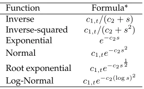
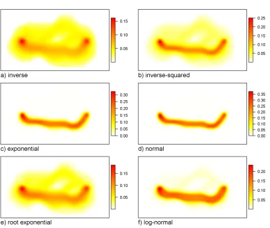
probability values. There are, however, many potential mathematical functions that could be used to definePi,t(see Table 3.1 which is developed after [15, 50]). The most
straight-forward way to model movement probabilities in the field-based space-time prism is to estimate the probability the individual visited locationi at timet as proportional to the inverse of the time deviation. However, [17] discusses the growing trend to use inverse-squared functions, typically in spatial interaction models. Alternatively, negative exponen-tial functions have the firmest theoretical foundation for modeling the decreasing activities as a function of distance, cost or time [16, 17, 54].
Function Formula*
Inverse c1,t/(c2+s) Inverse-squared c1,t/(c2+s2) Exponential e−c2s Normal c1,te−c2s
2
Root exponential c1,te−c2s
1 2
Log-Normal c1,te−c2(logs)
[image:5.612.239.387.285.376.2]2
Table 1: Potential functions used to derive probabilities from∆Ti(t)in field-based time
geography. *c1,tis a time-varying scaling parameter,c2is a time-decay tuning parameter
ands= ∆Ti,t.
In Table 3.1, the scaling parameterc1,tis used to standardize thePi,tso thatPPi,t = 1
at any timet. Scaling thePi,tis necessary to account for variations in the size and structure
of theP P St[46, 56].
c1,t= 1
P ∀jPj,t
, j∈P P St (2)
The tuning parameter(c2 >0)is a decay parameter controlling the strength of the decay
function (from Table 3.1). Lower values (c2 ≈ 0) are used to model weaker decay and
model locations deviating from the shortest-time path with higher probabilities. Higher values (c2 0) are associated with stronger decay and model locations deviating further
from the shortest-time path with much lower probabilities. In nearly all applied scenarios
c2 will be unknown, but can be empirically estimated from the data (e.g., GPS tracking
data) using, for example, a leave-one-out numerical estimation procedure (similar to that proposed by [19] for Brownian bridges).
Calculating the cumulative visit probability (Pi) for any location i over the entire time
interval betweentaandtbcan be done by integrating thePi,tover time.
Pi=
Z tb
ta
In practice, the integral in equation (3) is not easy to calculate, but can be approximated numerically by taking a set ofnkequally spaced times betweentaandtb(i.e.,ta < tk < tb)
and performing numerical integration using the trapezoid rule.
Pi =
tb−ta
nk+ 1
X
∀tk
Pi,tk+
A
2
!
(4)
whereAis what is termed the anchor raster which is defined as 1 in the cells associated with the two anchors and 0 elsewhere. For any space-time prism the sum of thePiis equal
to the time budget of the prism, that isPP
i = tb−ta. This definition ofPiis powerful
because it facilitates easy interpretation of modeled probabilities relative to the overall time budget and can be interpreted as theexpected value of timespent at each location or can be considered as relative visit probabilities (as in a Brownian bridge, [19]). The map of the
Pifor the entire space-time prism represents the probabilistic version of the potential path
area — the projection of the space-time prism onto the spatial plane.
3.2
Factoring in anchor location uncertainty
Anchor points are subject to location uncertainty, typically due to data collection technol-ogy, which adds a further complication to time geographic analysis. Here, anchor un-certainty is incorporated by assuming that location error can be quantified by a bivariate Gaussian distribution. A bivariate Gaussian filter, with varianceσ2, is applied to the
re-sultingPi,tvalues. The parameterσis used to quantify the level of uncertainty associated
with he anchor point locations in a similar fashion to what is done with Brownian bridge models [19].
σ2t =δt2+ (1−δt)2
σ2 (5)
whereδtis defined as in (1). The function in equation (5) modelsσt2as time varying
be-tween anchor points. As time moves away from the anchorsσ2
tdecreases to a minimum at
the mid-point between the two anchors. Modeling location uncertainty dependent on time provides the desirable effect that as the object moves away from anchor points the location uncertainty has a lesser effect on the modeled movement probabilities, because location uncertainty is most important where actual location data exists (i.e., at the anchors). The modeling of location uncertainty in this way in effect smooths the outputPi,tvalues, with
the degree of smoothing dependent onσ, the effect of this parameter is further examined in the following demonstrations.
3.3
Implementation in R
The implementation of the algorithm described above is reproduced using equations (1-5). ThePi,tare computed recursively for an arbitrary numbernkof time points betweentaand
tb. ThePiare then computed from equation (3) via numerical integration and the trapezoid
approximation. Increasingnkleads to more precise estimates of the integral in equation (3)
(see Supplementary Material). A function is provided that facilitates the leave-one-out numerical estimation of thec2 parameter. The computational speed of the algorithm is
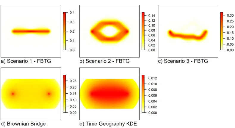
Figure 1: Three scenarios used to test field-based time geographic model; a) corridor, b) circular barrier, c) heterogeneous landscape.
in the statistical software R [51] as a set of functions as part of thewildlifeTG(Time geo-graphic analysis of wildlife movement) package available via GitHub [30]. The algorithm draws heavily on the previously developed packages for spatial analysis and cost surface analysis in R, most notably thegdistancepackage [53].
3.4
Three example scenarios
Three synthetic example scenarios are used to demonstrate the new field-based time geog-raphy model for estimating movement probabilities within the space-time prism. The first scenario represents the case where a corridor separates the two anchor points. The second scenario represents the case where a circular barrier is situated between the anchors A and B. The third scenario represents the more realistic case of movement through a heteroge-neous environment. The scenarios are represented on a 100x200 grid, where location A is at position (40,50) and location B is at position (160,50). The time budget for movement between A and B is 200 time units and nk = 200. The R code for generating the three
scenarios is provided as supplementary material.
As a spatial comparison,Pisurfaces are compared between field-based time geography
(c2 = 1, σ = 2), the Brownian bridge, and time-geographic kernel density estimation via
raster differencing to assess differences between the methods in terms of output probabili-ties. For the Brownian bridge and time geographic KDE models, the resulting probability surfaces were scaled so thatPP
i = 1(i.e., comparing probability densities). The distance
between any two surfaces is calculated as the Bhattacharyya distance (DB) [3] defined as:
DB(r1, r2) =−log
X√
r1r2
(6)
wherer1andr2are respectivePisurfaces to be compared. TheDB = 0when two surfaces
are identical and increases unbounded with increasing distance between the two surfaces. Output Pi surfaces can also be examined with respect to the most probable location
of movement at any given time (i.e., the location of the maximum value of Pi,t – or the
peak of the surface – termedlt). For both Brownian bridge and time geographic kernel
density estimation thelt locations are equivalent to the linear interpolation between the
anchors or more specifically, equally spaced points that follow the straight line from A to B [29]. However, for field-based time geography, theltlocations will follow closely along
a spatial and temporal measure of similarity between the two surfaces the Euclidean dis-tance betweenltlocations from field-based time geography is compared to the linear path
(associated with thelt locations from both Brownian bridges and time geographic kernel
density estimation) for each of the three scenarios.
3.5
Comparing the different parameter combinations
The selection of different input parameters will inevitably influence model results in field-based time geography. The cost surface defined by scenario 3 (Figure 1c) is used to test dif-ferences between different parameter combinations for computing the outputPisurfaces.
First, the functions for calculating thePi (i.e., those in Table 3.1) are compared visually in
terms of their output surfaces, and quantitatively using the Bhattacharya distance and dis-tance from theshortest time path. Second, differences between different values of the tuning parameterc2= [0.01, 0.1, 1] andσ= [0, 2, 4] (in pixel units) are evaluated. In evaluating
c2andσthe exponential model is presented (as similar results were observed for the other
models) and analysis is restricted to visually comparing differences betweenPi surfaces
from different parameter combinations. Finally, the choice ofnk and the pixel resolution
of the underlying surface are evaluated in order to assess the impact of the spatial and temporal granularity of analyisis.
3.6
Computational speed of the algorithm
The computational speed of the algorithm is examined by testing various parameter choices for each of the four key parameters: the number of intermediate time slices (nk),
the size of the raster grid (i.e., number of pixels) used to generate the cost surface, the magnitude ofσ, and the choice of time weighting function. Thenk are varied from 10 to
10,000, the size of the raster grid is varied from 4,000 to 4,000,000 pixels, the magnitude of
σis varied from 0 to 10 (in pixel units), and all six of the time-weighting functions (from Table 3.1) are evaluated (n= 10times). In each test, only one parameter is varied and the other three are held constant.
4
Results
4.1
Three example scenarios
Simply visualizing the output probability surfaces (i.e., the maps of thePi) provides an
initial assessment of field-based time geography in comparison to the other approaches (Figure 2). In particular, field-based time geography model estimates a uniquePisurface
for each scenario, whereas the Brownian bridge and time geographic density estimation models result in the same Pi surfaces regardless of the scenario (Figure 2). Time
geo-graphic kernel density estimation results in the lowest maximum probability value (and lower variation in output surface values) compared to field-based time geography and Brownian bridge outputs. Whereas the range of values is comparable between field-based time geography and Brownian bridge methods (based on the parameters used here).
Figure 2: a) - c) Output probability surfaces (Pi) from the three scenarios using the
field-based time geography model, d) the Brownian bridge model, and e) time geographic kernel density estimation.
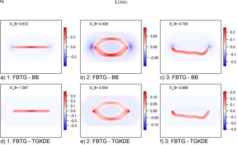
(DB = 0.872) and time geographic kernel density estimation (DB = 1.097) comparisons,
which might have been predicted to be the most similar based on visual assessment of the output UDs from (Figure 3). The difference map for Scenario 2 clearly demonstrates how the field-based time geography model captures avoidance of the barrier, while this is not the case for the Brownian bridge and time geographic kernel density estimation models. The distance between Pi surfaces for the field based time geography and the other two
methods was lowest (Figure 3 b & e). In scenario three, higherDB values were observed
(Figure 3 c & f) suggesting, very different surfaces between field-based time geography and the other two methods. TheDB= 0.059between the Brownian bridge and time geographic
kernel density estimation, which is substantially lower than for the comparisons with field-based time geography suggesting that Brownian bridge and time geography kernel density estimation methods result in, relatively, more similarPisurfaces when compared to
field-based time geography.
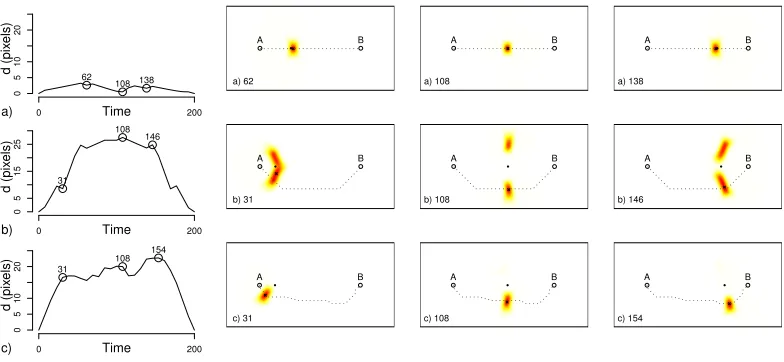
The distance (in pixel units) between the most probable location (lt) of field-based time
geography and a linear interpolation demonstrates some notable differences (Figure 4). First, in scenario 1 (Figure 4a) it would be expected that there is little differences here as both follow the direct route between the two anchors, however, due to resistance during the middle portion of the corridor, the deviations from zero are a result of changes in move-ment speed. With the second scenario (Figure 4b) it can be seen that the field-based time geography model adequately captures the barrier, and theltlocations are associated with
[image:9.612.117.512.111.327.2]Figure 3: Differences in thePi surfaces for each of the three scenarios. Tiles a) to c) show
based time geography against the Brownian bridge model and tiles d) - f) show field-based time geography against the time geographic kernel density estimation model. The Bhattacharyya distance (DB) is an overall measure of dissimilarity between the two
sur-faces ranging from 0 to 1 (whereDB = 0implies identical surfaces).
in the third scenario (Figure 4c) we see that the maximum difference inltoccurs at time
t= 154, and the deviation from linear interpolation varies considerably over time.
4.2
Comparing the different parameter combinations
The different functions (Table 3.1) for computingPiresulted in differentPisurfaces (Figure
5). The exponential and normal models (see Figure 5b-c) showed the steepest distribution and resulted in the largest maximum values. The inverse, root exponential and log-normal models all resulted in a less peaked distribution surface, with a lower maximum value of
≈ 0.3 (Figure 5a,e,f). The surfaces showed varying levels of similarity when evaluated usingDB, and pairwise comparison of each of these surfaces showed thatDBranged from
0.013 to 0.463 (Table 4.2). The exponential and normal models were the most similar, while the inverse and normal models were the most dissimilar (for the parameter combinations chosen here; Table 4.2).
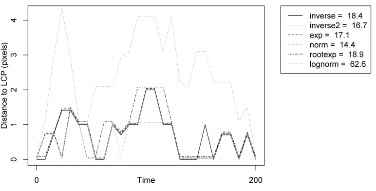
None of the methods for computingPiresulted inltlocations that deviated from the
least-cost path by more than about 4 pixels (Figure 6). The log-normal model deviated furthest from the least-cost path of all six methods, with maximum deviations of 3 to 4 pixels (Figure 6). The other five methods had more or less similar results withltlocations
deviating from the least-cost path by up to 2 pixels.
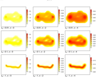
The effects of the tuning parameterc2and locational uncertainty parameterσwere also
Time d (pix els) 0 200 0 5 10 20 62 108 138 a) A B a) 62 A B a) 108 A B a) 138 Time d (pix els) 0 200 0 5 15 25 31 108 146 b) A B b) 31 A B b) 108 A B b) 146 Time d (pix els) 0 200 0 5 10 20 31 108 154 c) A B c) 31 A B c) 108 A B c) 154
Figure 4: Distance of the location of highest probability (lt) from the field-based time
ge-ography model to the linear interpolated path (the bee-line) for each of the three scenarios. ExamplePi,tsurfaces showtime-slicesof the field-based space-time prism associated with
specific time points during the segment.
Inverse Inverse2 Exponential Normal RootExp LogNorm
Inverse 0.000 0.067 0.376 0.463 0.025 0.252
Inverse2 0.000 0.111 0.160 0.017 0.060
Exponential 0.000 0.013 0.218 0.025
Normal 0.000 0.294 0.072
RootExp 0.000 0.123
LogNorm 0.000
Table 2: Bhattacharyya distance (DB) comparing different functions for deriving
proba-bilities from ∆Ti(t)in field-based time geography as applied to Scenario 3 (DB = 0for
identical surfaces).
thec2value is increased the output surface is more peaked and the probability density is
confined closer to the shortest time path. Very low values ofc2spread the distribution more
evenly across locations contained within the potential path space. The location uncertainty parameter results in a similar pattern, where higher values ofσresult in a smoother output
Pisurface.
The granularity of the analysis in terms of the choice of thenkparameter and the pixel
resolution of the underlying cost surface can significantly influence the resultingPisurface
(see Supplementary Material). As would be expected, lowernkvalues result in a less
con-tinuous outputPisurface and blocky artefacts are present at smallnkvalues. The output
surface appears comparatively smooth at much higher values fornk. Similarly, a coarser
pixel size results in a much coarser Pi surface while a finer pixel size results in a much
Figure 5: Output probability surfaces (Pi) from the six potential functions (see Table 3.1)
using the field-based time geography model applied to Scenario 3.
4.3
Computational speed of the algorithm
The field-based time geography algorithm as implemented is linearly dependent on both the user-defined number of time slicesnk(Figure 8a) and on the size (number of pixels) of
the raster grid upon which the calculation is conducted (Figure 8b). The locational uncer-tainty parameter (σ) showed a substantial increase in computation time in changing from
Figure 6: Distance (number of pixel units) of the location of maximum probability (lt) from
theshortest time pathfor each of the six potential functions (see Table 3.1) using the field-based time geography model applied to Scenario 3.
5
Case study: Wildlife movement analysis
5.1
Deriving the conductance surface
Figure 7: Output probability surfaces (Pi) for different values of the tuning parameterc2
and locational uncertainty parameterσusing the exponential model applied to Scenario 3.
5.2
Calculating the utilization distribution
The field-based time geography model requires the definition of four key parameters prior to implementation: 1) the mathematical time-decay model (i.e., from Table 3.1), 2) the num-ber of time slices to use in the algorithm (nk), 3) the location uncertainty parameter
(associ-ated with the telemetry data), and 4) thec2time-decay tuning parameter. The exponential
model was chosen for this analysis based on it’s widespread adoption in the geographical analysis literature and its performance in the initial tests described above. It is important to note that it is the choice ofc2 that is the most important. The number of time slices
was chosen to benk = 100 based on the earlier findings and in consideration of
computa-tional speed. The location uncertainty parameter associated with the telemetry data was chosen conservatively to be 100 m, which relates directly to the spatial resolution of the conductance surface. Finally, an empirical estimate of thec2parameter was derived from
the telemetry data using a similar leave-one-out optimization procedure to that described in [19]. The procedure generates a log-likelihood estimate for a user-defined range of val-ues and from which a value forc2= 0.002 was selected as optimal. The outputPisurface
Figure 8: Computational speed of the field-based time geography algorithm (as currently developed) when varying a) the number of time slices parameter (nk), b) the raster size
(spatial resolution, c) theσvalue (in number of pixels), and d) the choice of thePifunction.
To compare, the Brownian bridge utilization distribution [19] was also computed using thekernelbbfunction in the ’adehabitat’ package [4]. The movement variance parame-ter (σ2) was estimated using thelikerfunction following the methods described in [19].
The location uncertainty was set to 100 m. All surfaces were normalized to sum to 1 for comparison and presented as the√UD to better show the distribution of values. The 99% volume contour of the UD raster was used to delineate a home range polygon for both the field-based time geography and Brownian bridge methods for further comparison.
5.3
Case study results
The utilization distribution (Pisurface) produced by the field-based time geography is very
similar to that of the Brownian bridge (Db= 0.028; Figure 10a-c) and only small deviations
Figure 9: Data used in caribou example: a) slope (degrees) derived from a digital elevation model (DEM) of the study area, b) land cover data for the study area, and c) the derived conductance surface.
area in the middle of Figure 10d). In particular, the Brownian bridge assumes movement directly across a large lake, while the field-based time geography model is able to capture this barrier directly into the resulting UD and home range estimates. The ability of the field-based time geography model to capture both hard (such as lakes) and soft (such as variations in landcover/slope) barriers to movement is evident in the results of the caribou case study.
6
Discussion
Figure 10: Utilization distributions for a single caribou during the summer (July-August) of the year 2000 using the a) field-based time geography, and b) Brownian bridge methods, along with the 99% volume contour home ranges; c) the difference between the field-based time geography and Brownian bridge methods, and d) the home range polygons overlaid on the conductance surface of the study area with the caribou relocation points.
path, based on an underlying cost surface. This development is significant; probabilistic time geography was developed with the idea that within space-time prisms movement opportunities were unequal, and thus attempted to model these probabilistically using random walks. However, random walks are poorly suited for most applications, thus field-based time geography offers a more realistic alternative for scenarios where an appropriate cost surface can be defined. Moreover, field-based time geography explicitly consider the time limitations on movement in the construction of probabilistic space-time prisms.
Six different functions have been proposed for estimating the movement probabilities (i.e., Table 3.1) from the accumulated costs (or times) associated with a movement segment. Each of the functions represent a decay function used to convert the deviation in time from the shortest cost path (∆Ti,t) into movement probabilities, taking a similar approach to that
employed with time geographic kernel density estimation [10]. Based on the results from the three scenarios, the normal model and exponential model were most similar, whilst the normal model and the inverse model were most dissimilar (based on the chosen parame-ters). This is not surprising as these different models have been universally employed in many classical spatial interaction models [12] and spatial interpolation [5]. However, fur-ther examination of the tuning parameterc2suggests that the choice ofc2is what controls
the shape of the output probability surface (see Figure 7), rather than the choice model function. A similar effect if found in traditional kernel density estimation, which is com-monly used to estimate the underlying probability surface from a sample of spatial points, where the kernel shape is far less important than the choice of the kernel bandwidth [45]. Estimating thec2parameter (from some available trajectory data) is straightforward using
a leave-one-out estimation procedure (similar to that for the Brownian bridge model; [19]) and a tool for this is provided as part of the accompanying R package.
The granularity of analysis, both spatial and temporal, is an important consideration when implementing field-based time geography models. The temporal granularity is as-sociated with the choice of the number of intermediate time slices (nk) upon which to base
the calculation. This parameter can significantly influence the output results, specifically, whennk is too small, it can result in unrealistic discontinuities in the outputPi surfaces
(Supplementary Material). Thus, it is important thatnkbe sufficiently large to avoid this
effect. However, the choice ofnk linearly increases computational time (Figure 5a). Thus,
the selection ofnk should be made by carefully weighing the computational costs whilst
avoiding values which are too low. The choice of spatial granularity (i.e., pixel size) will typically be a function of the underlying data used in the analysis (i.e., variables used to de-scribe the underlying resistance to movement). Coarser spatial granularities will be unable to capture fine-scale movement processes, whereas finer granularities may be unnecessarily costly in terms of computational speed (Figure 5b). Issues with spatial granularity are well known in least cost path analysis, specifically that when data are aggregated into coarser spatial resolutions the least cost path may be altered significantly [13, 44]. Thus, the effect of spatial resolution on output results should be considered carefully in relation to the scale of the movement process under study.
surface due to the fact that it is certain the object is located at the anchor points. A similar effect is noticed in Brownian bridge models when the location uncertainty parameter is set to≈ 0. In practice, the location uncertainty parameter will be based on the data and application, but in wildlife applications employing Brownian bridge models it is common to set the location uncertainty parameter to the standard deviation of the positional error associated with data collecting technology (e.g., GPS error; [19]).
Existing movement models for estimating movement probabilities based on random walks – notably Brownian bridges [19, 46] – are attractive because they treat the underly-ing movement process as stochastic. However, it is important to note that the estimates of movement probabilities that are derived from such models are deterministic. That is, given a set of parameters, for any pair of anchors with the same time budget and the same distance between them the output probability surfaces (i.e.,Pi’s) will be identical. This is
not the case with the field-based time geography model, as it is entirely dependent on the unique constraints imposed by the underlying environment – the context within which the movement occurs. Recent efforts have developed alternative models that consider context within a random walk framework [1], and are capable of similarly considering impedances to movement. Similarly, random walks can be readily incorporated into cost-path analysis in order to model so-called randomised shortest paths [42]. The additional development of randomised shortest paths into the field-based time geography framework can be readily implemented using existing functionality within the R packagegdistance[53], however, randomised shortest paths are similarly limited as with Brownian bridges in that they do not explicitly consider the temporal bounds of movement, and thus the development of truncated randomised shortest paths (similar to the truncated Brownian bridge of [46]) would be valuable.
The most significant potential application of field-based time geography is to the anal-ysis of wildlife tracking data. Use of field-based time geography offers new potential to improve and refine probabilistic measures of space use – commonly referred to as the uti-lization distribution(UD; [57]) where the UD is defined by combining each of thePisurfaces
for a larger telemetry dataset (the Case Study provides an example). Brownian bridges (and to a lesser extent time geographic kernel density estimation) represent the current state-of-the-art for estimating wildlife UDs. However, both the Brownian bridge and time geo-graphic kernel density estimation methods fail to capture the heterogeneous nature of the environments within which animals move. In applications involving terrestrial animals, field-based time geography might use slope, land cover, and anthropogenic barriers as vari-ables in defining an appropriate cost surface [28]. Similarly defining an appropriate cost surface for avian applications might depend on accurate wind speed measurements [43]. Importantly, following Long and Nelson [31, 33] field-based time geography can be used to highlight areas of commission error (areas that could not have been visited) in existing UD models, for example due to the presence of barriers [2] or the assumption of unrealistic movement speeds [33]. Quantifying barriers in individual-level wildlife movement is still a largely under-developed component in present wildlife movement models.
a space-time prism (for example with GPS tracking data). Given the prevalence at which individual-based tracking is now being used in the study of wildlife ecology [22], it will be important to identify ways field-based time geography can be used in wildlife space-use studies. Future work will develop field-based time geography for application specifically to the calculation of wildlife UDs.
Many studies are interested in studying human movement in non-network spaces where field-based time geography could be employed as an improved model of movement opportunities. For example, Kay [21] employed cost path analysis in their study of human route choices at an orienteering event in the United Kingdom, drawing on similar ideas first proposed by Douglas [8]. Similarly, there is increasing research on eco-tourism and field-based time geography might be used to model the potential movements of recreationalists such as hunters [48] and hikers [49] in a similar fashion to how terrestrial wildlife might be analyzed. Similarly, field-based time geography could be used to improve probabilistic models of missing person locations in wilderness search and rescue activities (e.g., [7]). Movement data associated with marine vessels could also benefit from the field-based time geography approach where barriers associated with land/shallow water, currents, and speed restricted zones could all be incorporated into the generation of a suitable cost surface. Further, the methods as described here could be applied to existing field-based time geography model along spatial networks (as presented by [37]) to derive movement probabilities based on resistance along the network (e.g., associated with traffic).
7
Conclusion
A new model for field-based time geography is presented where movement probabilities within the space-time prism are estimated from cost-path analysis, as is commonly em-ployed in two-dimensional lattices. When compared with two existing approaches – Brow-nian bridges and time geographic kernel density estimation – field-based time geography offers the distinct advantage of characterizing underlying factors that may restrict or limit movement opportunities. Specifically, the application of field-based time geography offers significant potential for studying wildlife movement and estimating utilization distribu-tions when wildlife move within heterogeneous environments where barriers are present – which is the case in nearly all potential applications. Similarly, there is significant potential to develop field-based time geography as an analysis tool to study human mobility outside of traditional transportation networks for example associated with outdoor recreational ac-tivity. The new field-based time geography method is implemented as part of an existing package in the free and open source statistical computing software R.
References
[2] BENHAMOU, S.,ANDCORNÉLIS, D. Incorporating movement behavior and barriers to improve kernel home range space use estimates. Journal of Wildlife Management 74, 6 (2010), 1353–1360. doi:10.2193/2009-441.
[3] BHATTACHARYYA, A. On a measure of divergence between two statistical populations defined by their probability distributions. Bulletin of the Calcultta Mathematical Society 35(1943), 99–109.
[4] CALENGE, C. The package "adehabitat" for the R software: A tool for the analysis of space and habitat use by animals.Ecological Modelling 197, 3-4 (2006), 516–519.
[5] CHANG, K.-T. Introduction to Geographic Information Systems, 5th ed. McGraw Hill International, New York, 2006.
[6] DELAFONTAINE, M., NEUTENS, T.,AND DEWEGHE, N. Modelling potential move-ment in constrained travel environmove-ments using rough space-time prisms.International Journal of Geographical Information Science 25, 9 (2011), 1389–1411.
[7] DOHERTY, P. J., GUO, Q., DOKE, J.,ANDFERGUSON, D. An analysis of probability of area techniques for missing persons in Yosemite National Park. Applied Geography 47 (2014), 99–110. doi:10.1016/j.apgeog.2013.11.001.
[8] DOUGLAS, D. H. Least-cost path in GIS using an accumulated cost surface and slope-lines.Cartographica 31, 3 (1994), 37–51. doi:10.3138/D327-0323-2JUT-016M.
[9] DOWNS, J. A.,AND HORNER, M. A. W. Probabilistic potential path trees for visu-alizing and analyzing vehicle tracking data. Journal of Transport Geography 23(2012), 72–80. doi:10.1016/j.jtrangeo.2012.03.017.
[10] DOWNS, J. A., HORNER, M. W., ANDTUCKER, A. D. Time-geographic density esti-mation for home range analysis.Annals of GIS 17, 3 (2011), 163–171.
[11] FANCY, S. G., AND WHITE, R. G. Energy expenditures for locomotion by barren-ground caribou.Canadian Journal of Zoology 65, 1 (1987), 122–128. doi:10.1139/z87-018.
[12] FOTHERINGHAM, A. S. Modelling hierarchical destination choice. Environment and Planning 18, 3 (1986), 401–418. doi:10.1068/a180401.
[13] GONÇALVES, A. B. An extension of GIS-based least-cost path modelling to the loca-tion of wide paths. International Journal of Geographical Information Science 24, 7 (2010), 983–996. doi:10.1080/13658810903401016.
[14] HÄGERSTRAND, T. What about people in regional science? Papers of the Regional
Science Association 24, 1 (1970), 7–21.
[15] HAGGETT, P., CLIFF, A. D., ANDFREY, A. Locational Models. Edward Arnold Ltd., London, 1977.
[17] HAYNES, R., LOVETT, A.,ANDSUNNENBERG, G. Potential accessibility, travel time, and consumer choice: Geographical variations in general medical practice registra-tions in Eastern England. Environment and Planning A 35, 10 (2003), 1733–1750. doi:10.1068/a35165.
[18] HIJMANS, R. J. raster: Geographic Data Analysis and Modeling. R package version 2.5-8. https://CRAN.R-project.org/package=raster, 2016.
[19] HORNE, J. S., GARTON, E. O., KRONE, S. M., ANDLEWIS, J. S. Analyzing animal movements using Brownian bridges.Ecology 88, 9 (2007), 2354–2363.
[20] JOHNSON, C. J., PARKER, K. L., HEARD, D. C.,ANDGILLINGHAM, M. P. Movement parameters of ungulates and scale-specific responses to the environment. Journal of Animal Ecology 71, 2 (2002), 225–235. doi:10.1046/j.1365-2656.2002.00595.x.
[21] KAY, A. Route choice in hilly terrain. Geographical Analysis 44, 2 (2012), 87–108. doi:10.1111/j.1538-4632.2012.00838.x.
[22] KAYS, R., CROFOOT, M. C., JETZ, W., AND WIKELSKI, M. Terrestrial animal
tracking as an eye on life and planet. Science 348, 6240 (2015), aaa2478–aaa2478. doi:10.1126/science.aaa2478.
[23] KOBAYASHI, T., MILLER, H. J.,ANDOTHMAN, W. Analytical methods for error prop-agation in planar space-time prisms. Journal of Geographical Systems 13, 4 (2010), 327– 354. doi:10.1007/s10109-010-0139-z.
[24] KRAAK, M. J. The space-time cube revisited from a geovisualization perspective. InProceedings 21st International Cartographic Conference(August 10-16, Durban, South Africa, 2003), pp. 1988–1995.
[25] KUIJPERS, B., MILLER, H. J., NEUTENS, T., ANDOTHMAN, W. Anchor uncertainty and space-time prisms on road networks. International Journal of Geographical Informa-tion Science 24, 8 (2010), 1223–1248. doi:10.1080/13658810903321339.
[26] KUIJPERS, B., MILLER, H. J., ANDOTHMAN, W. Kinetic space-time prisms. In19th ACM SIGSPATIAL International Conference on Advances in Geographic Information Sys-tems(Nov. 1-4, Chicago, IL, 2011), Association for Computing Machinery, pp. 162–170.
[27] KWAN, M. Gender and individual access to urban opportunities: A study using
space-time measures. Professional Geographer 51, 2 (1999), 210–227.
[28] LAPOINT, S., GALLERY, P., WIKELSKI, M., AND KAYS, R. Animal behavior, cost-based corridor models, and real corridors. Landscape Ecology 28, 8 (2013), 1615–1630. doi:10.1007/s10980-013-9910-0.
[29] LONG, J. A. Kinematic interpolation of movement data Kinematic interpolation of movement data. International Journal of Geographical Information Science 30, 5 (2016), 854–868. doi:10.1080/13658816.2015.1081909.
[30] LONG, J. A. wildilfeTG: Time geographic analysis of wildlife movement, 2017.
[32] LONG, J. A., AND NELSON, T. A. A review of quantitative methods for movement data. International Journal of Geographical Information Science 27, 2 (2013), 292–318. doi:10.1080/13658816.2012.682578.
[33] LONG, J. A., AND NELSON, T. A. Home range and habitat analysis using dynamic time geography. Journal of Wildlife Management 79, 3 (2015), 481–490. doi:10.1002/jwmg.845.
[34] LONG, J. A., NELSON, T. A.,ANDNATHOO, F. S. Toward a kinetic-based probabilistic time geography. International Journal of Geographical Information Science 28, 5 (2014), 855–874. doi:10.1080/13658816.2013.818151.
[35] MILLER, H. J. Modelling accessibility using space-time prism concepts within geo-graphical information systems.International Journal of Geographical Information Systems 5, 3 (1991), 287–301.
[36] MILLER, H. J. A measurement theory for time geography. Geographical Analysis 37, 1 (2005), 17–45.
[37] MILLER, H. J.,ANDBRIDWELL, S. A. A field-based theory for time geography.Annals of the Association of American Geographers 99, 1 (2009), 49–75.
[38] MILLER, H. J., AND SHAW, S.-L. Geographic Information Systems for Transportation: Principles and Applications. Oxford University Press, Oxford, UK, 2001.
[39] NEUTENS, T., SCHWANEN, T., WITLOX, F.,AND DEMAEYER, P. Evaluating the tem-poral organization of public service provision using space-time accessibility analysis. Urban Geography 31, 8 (2010), 1039–1064. doi:10.2747/0272-3638.31.8.1039.
[40] O’SULLIVAN, D., MORRISON, A., AND SHEARER, J. Using desktop GIS for the in-vestigation of accessibility by public transport: an isochrone approach. International Journal of Geographical Information Science 14, 1 (2000), 85–104.
[41] PULLINGER, M. G., AND JOHNSON, C. J. Maintaining or restoring connectivity of modified landscapes: Evaluating the least-cost path model with multiple sources of ecological information.Landscape Ecology 25, 10 (2010), 1547–1560. doi:10.1007/s10980-010-9526-6.
[42] SAERENS, M., ACHBANY, Y., FOUSS, F., AND YEN, L. Randomized shortest-path problems: two related models. Neural Computation 21 (2009), 2363–2404. doi:10.1162/neco.2009.11-07-643.
[43] SAFI, K., KRANSTAUBER, B., WEINZIERL, R., GRIFFIN, L., REES, E. C., CABOT, D.,
CRUZ, S., PROAÑO, C., TAKEKAWA, J. Y., NEWMAN, S. H., WALDENSTRÖM, J., BENGTSSON, D., KAYS, R., WIKELSKI, M., ANDBOHRER, G. Flying with the wind: scale dependency of speed and direction measurements in modelling wind support in avian flight.Movement Ecology 1, 1 (2013), 4. doi:10.1186/2051-3933-1-4.
[45] SILVERMAN, B. Density Estimation for Statistics and Data Analysis. CRC Press, New York, 1986.
[46] SONG, Y.,ANDMILLER, H. J. Simulating visit probability distributions within planar space-time prisms. International Journal of Geographical Information Science 28, 1 (2014), 104–125. doi:10.1080/13658816.2013.830308.
[47] SONG, Y., MILLER, H. J., ZHOU, X.,ANDPROFFITT, D. Modeling Visit Probabilities within Network-Time Prisms Using Markov Techniques. Geographical Analysis 48, 1 (2016), 18–42. doi:10.1111/gean.12076.
[48] STEDMAN, R., DIEFENBACH, D. R., SWOPE, C., FINLEY, J., LULOFF, A., ZINN, H., SANJULIAN, G.,ANDWANG, G. Integrating wildife and human-dimensions research methods to study hunters.Journal of Wiildlife Management 68, 4 (2004), 762–773.
[49] TACZANOWSKA, K., GONZÁLEZ, L. M., GARCIA-MASSÓ, X., MUHAR, A., BRAN
-DENBURG, C.,ANDTOCA-HERRERA, J. L. Evaluating the structure and use of hiking trails in recreational areas using a mixed GPS tracking and graph theory approach. Applied Geography 55(2014), 184–192. doi:10.1016/j.apgeog.2014.09.011.
[50] TAYLOR, P. J. Distance transformation and distance decay functions. Geographical Analysis 3, 3 (1971), 221–238. doi:10.1111/j.1538-4632.1971.tb00364.x.
[51] TEAM, R. C., ANDR DEVELOPMENTCORE TEAM. R: A language and environment for statistical computing. Tech. rep., R Foundation for Statistical Computing, Vienna, Austria, 2017.
[52] TOBLER, W. Three presentations on geographical analysis and modeling: Non-isotropic geographic modelling; Speculations on the geometry of geography; and global spatial analysis. Tech. rep., NCGIA Technical Reports (93-1), University of Cal-ifornia, Santa Barbara, CA, 1993.
[53] VANETTEN, J. gdistance: Distances and Routes on Geographical Grids (v 1.1-9). Tech.
rep., 2015.
[54] WILSON, A. A statistical theory of spatial distribution models. Transportation research 1, 3 (1967), 253–269. doi:10.1016/0041-1647(67)90035-4.
[55] WINTER, S., AND YIN, Z. Directed movements in probabilistic time geogra-phy. International Journal of Geographical Information Science 24, 9 (2010), 1349–1365. doi:10.1080/13658811003619150.
[56] WINTER, S.,ANDYIN, Z. The elements of probabilistic time geography.Geoinformatica 15, 3 (2011), 417–434. doi:10.1007/s10707-010-0108-1.
[57] WORTON, B. Kernel methods for estimating the utilization distribution in home-range studies.Ecology 70, 1 (1989), 164–168.
[59] ZIPF, G.Human Behaviour and the Principle of Least Effort. Addison-Wesley Press, Cam-bridge, MS, 1949.
A
Example: Caribou telemetry data in Northern BC, Canada
A.1
Loading and viewing the data
This example will demonstrate the use of field-based time geography to estimate the uti-lization distribution(UD) of an animal which is a common spatial measure of movement and typically used to study the animal’s home range.
Three key datasets are included as part of the supplementary material found at https://github.com/jedalong/wildlifeTG.
• m3—the telemetry data for the caribou over the summer season,
• dem—a digital elevation model clipped to the study area,
• eosd—a land cover dataset (see [58]) clipped to the study area.
First we will use the DevTools package to load in the wildlifeTG package from it’s repos-itory on GitHub. The three datasets are stored within the package.
library(devtools)
install_github("jedalong/wildlifeTG")
library(wildlifeTG)
First, let’s take a look at the caribou telemetry data (Figure 11). The telemetry data was recorded using satellite collars, where a position fix was attempted every 4 hours. These data are for the individual “M3” and were recorded during the year 2000. Here we are only going to focus on the summer season which is defined as the months of July and August. In total there are n = 327 fixes in the dataset. The data is stored as anltrajobject from the packageadehabitatLT[4].
library(adehabitatLT)
data(m3) plot(m3)
Next, we will look at the DEM and land cover data (Figure 12). The DEM and land-cover data have both been resampled to a resolution of 100m, which is adequate for this demonstration (and given the large study area seems appropriate). Both datasets have also been clipped to the area surrounding the caribou telemetry data, so as not to include ex-tra area in the analysis and improve the speed of computation. The data are stored as a
RasterLayerobject from the packageraster[18].
library(raster)
data(dem) data(eosd)
par(mfcol=c(1,2),mar=c(4,4,4,6)) plot(dem)
Figure 11: Output of plot(m3).
A.2
Generating the cost surface
We are going to use Tobler’s hiking function [52] combined with empirical findings on cari-bou mobility [11] to generate the impact of slope (in degrees) on movement by caricari-bou. We need to generate a conductance surface where the value in each pixel reflects how quickly that pixel can be traversed by a caribou. We start by focusing solely on slope, where To-bler’s hiking function is adjusted so that a maximum of 4.5 km/h is used (based on the findings by [11]). We need to use thegdistancepackage [53] here.
library(gdistance)
altDiff <- function(x)x[2] - x[1]
speed <- transition(dem, altDiff, 8, symm=FALSE) speed <- geoCorrection(speed)
adj <- adjacent(dem, cells=1:ncell(dem), pairs=TRUE, directions=8)
#Tobler’s hiking function (modified)
speed[adj] <- (4.5/3.6)*exp(-3.5 * abs(speed[adj] + 0.05))
Figure 12: Output of plot(dem) and plot(eosd).
m <- matrix(c(0,12.5,1, #NoData
19,21,0.1, #Water
30,31.5,0.5, #Snow
31.5,32.5,0.5, #Rock
32.5,33.5,1, #Bare
39.5,49,1, #Bryoids
49.5,59,1, #Shrubs
80,81.5,0.8, #Wetland - Treed
81.5,83.5,0.5, #Wetland
99,101,1, #Herbs
200,240,0.8 #Trees - various
),ncol=3,byrow=T)
eosd <- reclassify(eosd,m)
gd <- transition(eosd, mean, 8, symm=FALSE) speed[adj] <- speed[adj]*gd[adj]
speed <- geoCorrection(speed)
Figure 13: Output of conductance surface.
whiteish areas), the areas associated with steep mountains having lower conductance (in brown) and the areas that facilitate easier movement (in green).
ras <- raster(speed) plot(ras)
We can also add the telemetry points on top (Figure 14).
plot(ras)
points(ld(m3)$x,ld(m3)$y,pch=20,cex=0.8)
A.3
Computing the field-based time geographic UD
First we need to set up the parameters of the analysis. Specifically we need to define:
• c2—The time-decay tuning parameter.
• nk—The number of time-slices used by the algorithm.
• σ—The location uncertainty parameter (associated with the telemetry data).
• The mathematical function used to implement the time-decay model, one of:
– inverse
Figure 14: Output of conductance surface with telemetry points.
– root-exponential – normal
– log-normal
We will usenk=100 as a fairly good default for the number of time-slices. The location
uncertainty for this data (satellite tags) is assumed to be about 100m so we will setσ=100. We will use the “exponential” model as the time-decay function. We will use a provided function (namedestc2) to computec2using a “leave-one-out” estimation procedure. The estc2function produces a curve identifying an optimized (maximum likelihood)c2
pa-rameter value based on the estimation procedure (Figure 15). Here based on previous runs of the function, the maximum value of 0.01 is used (which means we are estimatingc2
between 0 and 0.01).
n_k <- 100
sigma <- 100
timefun <- ’exp’
#Note: this function is slow (˜ 2 minutes).
c_2 <- estc2(m3,speed,timefun=timefun,max=0.01)
Here we can see for this example that the optimizedc2 value is 0.0018367. Once we
have estimatedc2from the data we are ready to implement the field-based time geography
Figure 15: Output of conductance surface with telemetry points.
t1 <- Sys.time()
m3ud <- fbtgUD(m3,speed,c2=c_2,sigma=sigma,timefun=timefun, k=n_k,clipPPS=F)
#Note: this function is very slow (30 mins!)
t2 <- Sys.time()
difftime(t2,t1,units=’mins’)
The sum of the output UD pixel values is equal to the entire time budget of the animal?s tracking period (i.e.,tn−t1).
cellStats(m3ud,sum)/(60*60*24) #Convert seconds to days
We will take a look at the output UD in a plot, and we can also plot the square root of the UD to get a better look at the values (Figure 16). The output is a raster which will sum to the time budget of the entire trajectory (i.e., the difference in time between the first and last fix).
par(mfcol=c(1,2),mar=c(3,3,3,6)) plot(m3ud)
plot(m3udˆ0.5)
Figure 16: Output UD and square root of UD.
hr95 <- volras(m3ud,95) plot(m3ud)
plot(hr95,add=T)