Studying Effect of Magnetizing Curve Nonlinearity Index on the Occurring Chaotic Ferroresonance Oscillation in Autotransformers

doi:10.4236/epe.2011.32011 Published Online May 2011 (http://www.SciRP.org/journal/epe)

Studying Effect of Magnetizing Curve Nonlinearity Index

on the Occurring Chaotic Ferroresonance Oscillation in

Autotransformers

Hamid Radmanesh1, Mehrdad Rostami2, Jafar Khalilpour1

1

Electrical Engineering Department, Shahid Sattari Aeronautical University of Science & Technology, Tehran, Iran

2

Electrical Engineering Department, Shahed University, Tehran, Iran

E-mail: hamid.radmanesh@aut.ac.ir, Rostami@shahed.ac.ir, j_khalilpour@yahoo.com Received December 31, 2010; revised March 7, 2011; accepted March 15, 2011

Abstract

This paper investigates the effect of iron core saturation characteristic degree on the onset of chaotic ferrore-sonance and duration of transient chaos in an autotransformer. The transformer chosen for study has a rating of 50 MVA, 635.1 kV, the magnetization characteristic of the autotransformer is modeled by a single-value two-term polynomial with q = 5, 7, 11. The core loss is modeled by a linear resistance and is considered a fix value for it. Simulation results are derived by using MATLAB software and nonlinear dynamics tool such as bifurcation and phase plan diagrams. It is shown settling down to the chaotic region is increased when degree of core nonlinearity is gone from 5 to 11.

Keywords:Linear Core Losses, Chaotic Ferroresonance, Bifurcation Diagrams, Autotransformers

1. Introduction

Ferroresonance is initiated by improper switching opera-tion, routine switching, or load shedding involving a high voltage transmission line. It can result in Unpredictable over voltages and high currents. The prerequisite for fer-roresonance is a circuit containing iron core inductance and a capacitance. Such a circuit is characterized by si-multaneous existence of several steady-state solutions for a given set of circuit parameters. The abrupt transition or jump from one steady state to another is triggered by a disturbance, switching action or a gradual change in val-ues of a parameter. Typical cases of ferroresonance are reported in [1-4]. Theory of nonlinear dynamics has been found to provide deeper insight into the phenomenon. In [5,6] is among the early investigations in applying theory of bifurcation and chaos to ferroresonance. The suscepti-bility of a ferroresonance circuit to a quasi-periodic and frequency locked oscillations has been presented in [7]. In this case, investigation of ferroresonance has been done upon the new branch of chaos theory that is qua-siperiodic oscillation in the power system and finally ferroresonance appears by this route. Effect of initial conditions on occurring ferroresonance oscillation is

2. Circuit Descriptions and Modeling

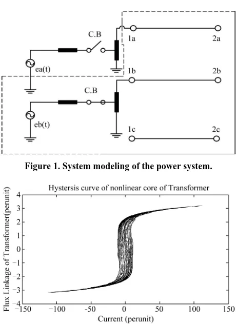
Three-phase diagram for the circuit is shown in Figure 1.

The 1100 kV transmission line was energized through a bank of three single-phase as reported in autotrans-formers. Ferroresonance occurred in phase A when this phase was switched off on the low-voltage side of the autotransformer; phase C was not yet connected to the transformer at that time [17]. The autotransformer is modeled by a T-equivalent circuit with all impedances referred to the high voltage side. The magnetization branch is modeled by a nonlinear inductance in parallel with a nonlinear resistance and these represent the nonlinear saturation characteristic, and nonlinear hys-teresis curve [17]. Iron core saturation characteristic is given by:

q Lm

i ab (1)

The exponent q depends on the degree of saturation. It was shown that for proper representation of the satura-tion characteristics of a power transformer the exponent q may take the values 5, 7, and 11. In this paper, the core losses model is described by a linear resistance. The polynomial of order seven and the coefficient b of

Equa-tion (1) are chosen for the best fit of the saturaEqua-tion region. It was shown in this paper that for lower order polyno-mials, chaos occurred for larger value of input voltage, also for polynomials of order 5 and 7, chaos did not ap-pear for low losses and only fundamental and subhar-monic resonances are obvious.

Figure 2 shows the hysteresis curve of the iron core of

the auto transformer that is simulated and obtained for the transformer that is studied in this paper. It is thus important to have as accurate an approximation to the magnetization curve as possible.Because of the nonlin-ear nature of the transformer magnetizing characteristics, the behavior of the system is extremely sensitive to change in system parameter and initial conditions. A small change in the value of system voltage, capacitance or losses may lead to dramatic change in the behavior of it. A more suitable mathematical language for studying ferroresonance and other nonlinear systems is provided by nonlinear dynamic methods. Mathematical tools that are used in this analysis are phase plan diagram, time domain simulation and bifurcation diagram.

The circuit in Figure 1 can be reduced to a simple

form by replacing the proposed power system with the thevenin equivalent circuit as shown in Figure 3. Figure 4 shows the equivalent circuit of the power system

in-cluding auto transformer that is derived by applying thevenin theorem to the initial single line diagram of the power system. By using the steady-state solution of MATLAB SIMULINK with the data of the 1100 Kv

Figure 1. System modeling of the power system.

Figure 2. Hystersis curve of the iron core of the auto- transformer.

Figure 3.Thevenin circuit of the power system that is shown in Figure 1.

81

transmission line [17], Eth and zth were found to be:

th 130.1 kV; th 1.01243 0.5

E  z  j E 

2.1. Nonlinear Dynamics and Equation

The resulting circuit to be investigated is shown in Fig-ure 4 where Zth represents the Thevenin impedance. The

behavior of this power system can be described by the following system of nonlinear differential equations, by applying KVL and KCL laws to the circuit in the case of considering linear core losses effect can be driven as below:

th c 2 m L2 0 e v R i v v

       (2)

2 2 d d L i v L t

 (3) 1

d

c

v i t

C



_

2

th c 2 m L 0

e v R i v v

       (5)

0

d 1 1 d

d d

q c

m

v

a b h

t C R t

  

 

     

  (6)





d

q

Lm Rm

m

i i i a b

R t   

 

     

  (7)

2

2 1

2 2 2

d d d 1 d

d d d

q L

m

i

v L L a qb

t t dt R t

 _   

 

  _  _

  (8)

th 2

2

1

2 2

1 d d

.

d d

1 d d

d d q c m q m

e v R a b

R t t

L a qb d

R t t

 _{ }    _      _   _      _   _   (9)

The base values of the power system parameters are listed in Table 1.

Also, the per unit values of the nonlinear index coeffi-cients are listed in Table 2.

2.2. Simulation Results and Discussion

Ferroresonance in three phase systems can involve large power transformers, distribution transformers, or instru-ment transformers. The general requireinstru-ments for fer-roresonance are an applied or induced source voltage, a saturable magnetizing inductance of a transformer, a capacitance, and little damping. The capacitance can be in the form of capacitance of underground cables or long transmission lines, capacitor banks, coupling capacitances between double circuit lines or in a temporarily-un- grounded system, and voltage grading capacitors in HV circuit breakers. Other possibilities are generator surge

Table 1. Basic parameters value of the power system.

Vbase Ibase Cp.u Rp.u Rcore Rbase Lsp.u

635.1 kV 78.72 A 0.079 0.0014 556.68 8067 Ω 0.0188

Table 2. Different value of q with its coefficient.

q/coefficient A B

5 0.0071 0.0034e(–19)

7 0.000375 7.3824e(–24)

11 0.000375 1.5648e(–37)

capacitors and SVC’s in long transmission lines. Due to nonlinearities, increased capacitance does not necessarily mean an increased likelihood of ferroresonance. Operat-ing guidelines based on linear extrapolations of capaci-tance may not be valid. Also, as mentioned previously, the smaller the load on the transformer’s secondary, the less the system damping is and the more likely ferrore-sonance will be. Therefore, a highly capacitive line and little or no load on the transformer are prerequisites for ferroresonance. So, in the case of simulation, time do-main simulations were performed using fourth order Runge-Kutta method and validated against MATLAB SIMULINK, and effect of changing in the value of sys-tem capacitances doesn’t investigate in this paper. The initial conditions as calculated from steady-state solution of MATLAB are:

0,0;vm 1.67 pu;vC 1.55 pu

  

The circuit in Figure 4 is analyzed by first modeling

the core loss as a constant linear resistance. Simulation has been done in three categories, first: system simula-tion with linear core losses effect with considering de-gree of core nonlinearity q = 5, second system simulation

with linear core losses effect with considering degree of core nonlinearity q = 7 and finally investigation of

cha-otic ferroresonance by considering q = 11.

Figure 5 Shows the phase plan diagram of voltage and

flux linkage of the transformer with q = 5, according to

this plot, trajectory of the system has a chaotic behavior and over voltages of transformer reaches to 6 p.u. Cor-responding time domain simulation in Figure 6 clearly

shows the chaotic behavior of the voltage on the trans-former, value of time is considered as a per unit value and it is shows amplitude of this oscillation is reached to 5 p.u.

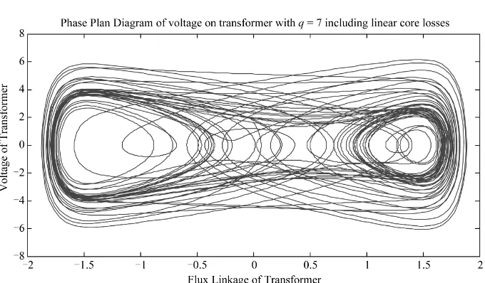
Figure 7 Shows the phase plan diagram of over voltage

on transformer with q = 7, it is shown when the degree of q increases from 5 to 7, amplitude of over voltage goes

Figure 5. Phase plan diagram for q = 5 considering linear core losses.

Figure 6. Time domain simulation for q = 5 considering linear core losses.

Figure 8 shows time domain simulation when input

voltage of the system is 4 p.u. This plot shows the cha-otic signal with much subharmonic resonance in it.

The circuit in Figure 4 is analyzed by first modeling

the core loss as a constant linear resistance. Figures 9

and 10 show the phase plan diagram and time domain

simulating with q = 11. It is shown that when q is

in-creased, nonlinear phenomena in the transformer are begun in the low value of the input voltage. It was shown that the chaotic behavior begins at a value of Ep = 2 p.u

for q = 5 and Ep = 1.5 p.u for q = 7, 11 where represents

the amplitude of eth(t). Another tool that can shows manner of the system in vast variation of parameters is bifurcation diagram. In Figure 11, voltage of the system

is increased to 8 p.u, and ferroresonance is begun in 2.5 p.u, it is shown that if input voltage goes up due to the abnormal operation or switching action, ferroresonance

phenomena is occurred. In Figure 11 input voltage is

increased up to 8 p.u and over voltage on transformer has been analyzed according to input voltage variation. In point (1) period 3 appears, in point (2) period 5 appears and jumping in the trajectory of the system has been take placed, in point (3) chaos has been begun and in point (4) system behavior comes out from chaotic region but there are many subharmonic resonance in the system. By re-peating simulation, between point (5), (6) and (7) again system has a nonlinear behavior. After the point (7) sys-tem has a periodic manner with the period 9 behavior.

Bifurcation diagrams in this paper are traced period doubling route to chaos and it is begun from period1, period 3, period 5 and by this manner goes to chaotic region. In the big value of input voltage, system behavior is completely nonlinear and chaotic over voltages reach to 3 p.u; this amplitude is very dangerous for transformer

Figure 8. Time domain simulation for q = 7 considering linear core losses.

Figure 10. Corresponding time domain signal that includes chaotic motion.

Figure 11. Bifurcation diagram for q = 5 considering linear core losses.

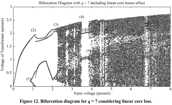
and can cause core failure. Figure 12. shows system over

voltage with q = 7. In this plot, one jump is occurred in

point (2), and chaos is appeared in point (3). By increas-ing degree of q, it is shown chaos appear in 2 p.u. by comparing this plot with the previous case, it is clearly shows ferroresonance oscillation is begun 0.5 p.u earlier than the case of considering q = 5.

Bifurcation diagram in Figure 13 shows more

nonlin-earity with q = 11, it is shown the chaotic overvoltage

after point (1) and period doubling oscillation is occurred in E = 1 p.u. Amplitude of this case is reached to 2.5 p.u.

Figure 13 shows system over voltage with q = 11,

ac-cording to this plot, in point (1), period 3 appears and in this point ferroresonance is begun. By comparing the bifurcation diagram in Figures 12 and 13 by Figure 11,

it is concluded that degree of nonlinear core can cause occurring the ferroresonance over voltages in the low

value of the input voltage. In the real system, when the input voltage due to the abnormal switching or other unwanted phenomena reaches to 4 p.u, transformer core is heated and can cause transformer core failure.

3. Conclusions

The dynamic behavior of an autotransformer is shown by the dynamical tool such as bifurcation and phase plan diagrams. In this paper, effect of changing the value of degree q on occurring ferroresonance over voltages is studied, and is shown the nonlinear iron core and its de-gree “q” has a great effect of occurring nonlinear

oscilla-tion in the autotransformer. When q is 11, chaotic over

85

Figure 12. Bifurcation diagram for q = 7 considering linear core loss.

Figure 13. Bifurcation diagram for q = 11 considering linear core loss.

in these transformers is more dangerous and should con-sider protecting tool on this transformers such as damp-ing resistor loads, MOV surge arrester and neutral earth resistance.

4. References

[1] H. W. Dommel, A. Yan, R. J. O. De Marcano and A. B. Miliani, “Tutorial Course on Digital Simulation of Tran-sients in Power Systems,” Chapter 14, IISc, Bangalore, 1983, pp. 17-38.

[2] E. J. Dolan, D. A. Gillies and E. W. Kimbark, “Ferrore-sonance in a Transformer Switched with an EVH Line,” IEEE Transactions on Power Apparatus and Systems, Vol. PAS-91, 1972, pp. 1273-1280.

[3] R. P. Aggarwal, M. S. Saxena, B. S. Sharma, S. Kumer and S. Krishan, “Failure of Electromagnetic Voltage

Transformer due to Sustained Overvoltage on Switch-ing*/an In-Depth Field Investigation and Analytical Study,” IEEE Transactions on Power Apparatus and Systems, Vol. PAS-100, No. 11, 1981, pp. 4448-4455.

[4] C. Kieny, “Application of the Bifurcation Theory in Studying and Understanding the Global Behavior of a Ferroresonant Electric Power Circuit,” IEEE Transac-tions on Power Delivery, Vol. 6, No. 2, 1991, pp. 866- 872.

[5] A. E. A. Araujo, A. C. Soudack and J. R. Marti, “Fer-roresonance in Power Systems: Chaotic Behaviour,” IEE Proceedings-C, Vol. 140, No. 3, 1993, pp. 237-240. [6] B. A. Mork and D. L. Stuehm, “Application of Nonlinear

and Quasi Periodic (QP) Oscillations in Power Systems,” IEEE Transactions on Power Delivery, Vol. 13, No. 2, 1997, pp. 560-569. doi:

[8] S. Mozaffari, M. Sameti and A. C. Soudack, “Effect of Initial Conditions on Chaotic Ferroresonance in Power Transformers,” IEE Proceedings of Generation, Trans-mission and Distribution, Vol. 144, No. 5, 1997, pp. 456- 460.

[9] S. Mozaffari, S. Henschel and A. C. Soudack, “Chaotic Ferroresonance in Power Transformers,” IEE Proceed-ings of Generation, Transmission and Distribution, Vol. 142, No. 3, 1995, pp. 247-250.

[10] B. A. T. Al-Zahawi, Z. Emin and Y. K. Tong, “Chaos in Ferroresonant Wound Voltage Ttransformers: Effect of Core Losses and Universal Circuit Behavioral,” IEE Pro-ceedings of Science, Measurement and Technology, Vol. 145, No. 1, 1998, pp. 39-43. [11] A. Rezaei-Zare, M. Sanaye-Pasand, H. Mohseni, Sh.

Farhangi and R. Iravani, “Analysis of Ferroresonance Modes in Power Transformers Using Preisach-Type Hysteretic Magnetizing Inductance,” IEEE Transaction on Power Delivery, Vol. 22, No. 2, 2007, pp. 919-928.

[12] K. Al-Anbarri, R. Ramanujam, T. Keerthiga and K. Kup-pusamy, “Analysis of Nonlinear Phenomena in MOV Connected Transformers,” IEE Proceedings of Genera-tion, Transmission and Distribution, Vol. 148, No. 6,

2001, pp. 562-566.

[13] H. Radmanesh, A. Abassi and M. Rostami, “Analysis of Ferroresonance Phenomena in Power Transformers In-cluding Neutral Resistance Effect,” SoutheastCon’09, IEEE, 1-5 March 2009, Atlanta, pp. 1-5.

doi:10.1109/SECON.2009.5233395

[14] H. Radmanesh and M. Rostami, “Effect of Circuit Breaker Shunt Resistance on Chaotic Ferroresonance in Voltage Transformer,” Advances in Electrical and Com-puter Engineering, Vol. 10, No. 3, 2010, pp. 71-77. http://dx.doi.org/10.4316/AECE.2010.03012.

[15] H. Radmanesh, “Controlling Ferroresonance in Voltage Transformer by Considering Circuit Breaker Shunt Re-sistance Including Transformer Nonlinear Core Losses Effect,” International Review on Modelling and Simula-tions, Vol. 3, No. 5, Part A,2010.

[16] H. Radmanesh and M. Rostami, “Decreasing Ferroreso-nance Oscillation in Potential Transformers Including Nonlinear Core Losses by Connecting Metal Oxide Surge Arrester in Parallel to the Transformer,” International Re-view of Automatic Control, Vol. 3, No. 6, 2010, pp. 641- 650.

[17] H. Radman

International Review of