An adaptive scheme for the efficient calculation of impedance loci

AN

ADAPTIVE SCHEME

FOR THE EFFICIENT CALCULATION

OF IMPEDANCE LOCI

by

I.D. Coope

Department of Mathematics, University of Canterbury, Christchurch, New Zealand

and

N.R. Watson and

J.

Arrillaga

Department of Electrical & Electronic Engineering, University of Canterbury,

Christchurch, New Zealand

No. 62 February, 1991

To appear in

AN ADAPTIVE SCHEME FOR THE

EFFICIENT CALCULATION OF

IMPEDANCE LOCI

I.D. Coope, N.R. Watson and

J.

Arrillaga

Abstract. Impedance loci information is well used by electrical engineers. In power system engineering it is useful too: (i) to see if the addition of static VAR compensation

will cause resonance problems; (ii) to enable harmonic filters to be designed and (iii) to

assess if a proposed ripple control frequency is practical. In the past, to obtain a good frequency locus, the frequency range was scanned using a constant but small increment in frequency. This is computationally very expensive and interpolation methods have also been used to allow a larger frequency increment in the scan. By allowing the interval between frequency points to vary a better choice of frequencies for impedance evaluation can be found. An adaptive scheme for automatically choosing the frequencies for impedance evaluation is described. A parametric cubic spline is then fitted through the chosen points. This dramatically reduces the number of frequency points that need to be evaluated without losing any essential detail in the loci.

1

Introduction

Impedance loci are important in determining the interactions of power system components. For

example:-• When designing harmonic filters for HVDC schemes, the system loci must be obtained for various system conditions. These are then used to assess the interaction with the proposed filters to ensure that the filters will perform adequately under the expected system conditions.

e Ripple control is extensively used by power utilities for a great number of functions. Examples include street lighting control, night rate metering and load management. The impedance locus is important to determine the best ripple frequency and whether proposed changes to the system will hinder the ripple signal from propagating sufficiently. A low impedance at the ripple frequency will generally mean that the ripple voltage resulting from the injection of ripple signal will be insufficient to operate reliably the ripple switches.

• Capacitor banks and static VAR units are used to supply MVARs and therefore reduce the line currents and losses. However, addition of such units can hinder ripple control

by absorbing too much ripple signal, or cause a harmonic resonance which if excited

To produce impedance loci, the harmonic response of each power system component must be assessed and the system admittance matrix formed. This matrix is then reduced to obtain the system impedance as seen from the observation busbar. In the past, the system impedance has been assessed by scanning the desired frequency range with a constant frequency interval

between evaluations[!, 2, 3]. In order to pick up the details in the regions where the impedance

is changing rapidly with frequency, a small frequency interval is required. However, this results in an excessive number of frequencies to evaluate the system impedance, and excessive computation time. Therefore, by allowing a variable frequency interval between evaluations, a small frequency interval can be used when the impedance is changing rapidly and larger intervals elsewhere.

2

The Sampling Problem

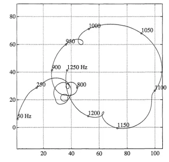
The impedance locus of an AC network is typified by the example in Figure 1, representing a model of the power system of the South Island of New Zealand, as seen from Benmore,

operating at 100% load. For the frequency interval 50 :::;

f :::;

1250 Hz, the resistance,

R(f),

and reactance, X(J), are plotted to give the spiral-like curve shown. In order to plot the

smooth curve of Figure 1, the system impedances were calculated at frequency intervals of 1 Hz and this curve is, therefore, taken to represent the modelled impedances to high accuracy throughout the given interval.

80 '''"'''''''"'''''''.'"''''"''''''''"''''t''''"''''''"""""j'"'''''''''"'''"''''!""""''""''''""':"'

: : :

60

···:···••!•••··· ·:···· _{. .}

. .

: :

: :

: :

: :

1iso

Hz

40 ... j ... : ... , ...

T

...

r ..

I

:

1

o

. .

20 .... , ... \

t

'

,

0 ... " """" j· .... " " ' " ' " ' " ' " " ! " " " " " """"""1"""""'

l.l:5.0 ...

~

.. .

: :

20 40

60

80 100

Resistance, R(f) ohms

[image:3.600.126.458.388.706.2]

It should be clear from inspection of the locus that it is wasteful to use such a small frequency increment between impedance evaluations over the whole range. The locus can be summarised much more efficiently by using small frequency increments where there are tight loops and much larger increments elsewhere. Because the loops correspond to resonances it is important to be able to display them accurately and the danger in using a larger frequency increment is that some loops may be missed completely. Of course, the real difficulty is that the positions

of the loops are not known until after the curve has been plotted. The sampling problem is,

therefore, that of choosing the frequencies at which the impedances are evaluated in a way that provides an efficient and accurate summary of the impedance locus.

Clearly, what is required is an adaptive scheme, capable of automatically adjusting the frequency increment according to the local geometry of the curve. When the curvature is large the impedance should be sampled at small frequency intervals and when the curvature is small it should be sufficient to sample at intervals which are larger, provided that the interval is not so large that complete loops are "smoothed away". Ideally then, it might be argued, that

the impedances should be calculated at frequencies

{/k,

k

=

1, 2, ... } such that

7/Jk+

1 - ·i/Jk

=

a,

where 1/Jk

=

1/J(Jk) is the angle between the tangent to the locus at the frequency fk and the

R-axis (or some other fixed line) and a represents a constant angle. This approach would

guarantee that small loops are given as much attention as large loops. For example, if the true

locus were a circle and if a were fixed at 45°, then the locus would be summarised by eight

equally spaced points around the circumference, irrespective of the radius of the circle.

The change in angle, 61/Jk

=

1/Jk+i - 1/Jk, as the frequency changes from fk to fk+i is

referred to as the winding angle and this will be negative for any sub-interval of the curve which has a clockwise orientation. The locus in Figure 1 has a clockwise orientation over most

of the range 50 ~

f

~ 1250 Hz. This is a characteristic of all impedance loci observed by

the authors. However, there are small regions where the angle of rotation winds in an anti-clockwise direction. Examples are in the regions near 250 Hz and 1100 Hz where it might be

thought that there should be extra tight loops. (In order to be reasonably confident that there

are no extra loops the locus was re-plotted using

t

Hz intervals with no discernible change in

the locus.) An adaptive scheme should adjust the frequency increment to a small setting in these regions not because the rate at which the winding angle changes is too high, but because it has an unexpected sign.

In order to be able to take advantage of the above observations in the design of an adaptive

sampling scheme it is necessary to have a simple means of estimating 61/Jk, the change in

tangent angle in moving from the point fk to fk+1 on the impedance locus. Then if this

estimate is too large the impedance should be evaluated again at some intermediate point, say

f

=

t(fk

+

fk+i)·

3

Estimating the Winding Angle

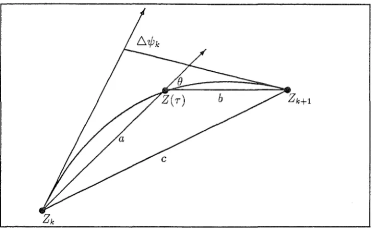
The diagram in Figure 2 represents a magnified view of a small portion of the impedance

locus. Suppose that the impedance Z(J)

=

R(J)

+

jX(J) has already been calculated at each

of two frequencies fk, fk+t· Then the angle through which the tangent to the curve winds as

the locus is traversed from Zk = Z(Jk) to Zk+1

=

Z(fk+1 ) can be estimated by evaluating the

impedance Z (

T)

at an intermediate point

T

in the interval

[f

k, f k+i

l ·

If 8 denotes the angle

between the chords Z ( T) - Z k and Z k+i - Z ( T) and if the locus has constant curvature over

the interval fk ~ f ~ fk+i, (i.e. it is a circular arc,) then some simple geometry shows that

is estimated well by W, if the curvature does not vary too much over the interval in question. Moreover, for a smooth locus (at least differentiable) the mean value theorem can be invoked

twice to show that the winding angle must be at least () on an interval that contains T and

which is a strict subset of the interval

[fk,

fk+d. In any event if the angle () is not small then

clearly more points are required if the locus is to be summarised well.

Figure 2. Estimating the winding angle, 61/;k, using the chord angle (),

The diagram in Figure 2 is appropriate only if B

<

go

0

• This situation is easily detected by

calculating the chord lengths a, b and c. If a2

+

_b2

_<

_c2 _{then the angle B is acute and 61/;k}

can be estimated by W; the smaller this angle the more accurate is the approximation. If

a

2

₊

_b

2 _{~ c}2 _{then it is not even worth calculating the angle}

_B,

_{clearly the points}

_{Zk, Z( r)}

_and

Zk+

₁

are spaced too far apart. In this case each of the sub-intervals

[fk,

r]

and

[r,

fk+1 ]

can

be processed separately by evaluating the impedance again at an intermediate frequency and estimating the winding angles on each new sub-interval.

The calculation of the chord lengths is not wasted when ()

<

goo,

because the lengths a, b

and c can be used to get estimates of the winding angles 61/;k,l and 61/;k,2 on each of the

sub-intervals. Again, some simple geometry provides the estimates:

61/Jk,1

=

arcsin(

~c

sin B), 61/Jk 2

=

arcsin(

~sin()),

' c

and it is straightforward to verify that these estimates satisfy 61/Jk,l

+

61/Jk,2

=

2(), as expected.

In fact the angle () can also be calculated from the chord lengths since it satisfies the equation

c2 - a2 - b2

cos 1e1 = b ,

2a

but it is preferable to calculate () in terms of the arctan function in order to preserve the orientation of the winding angle. The advantage in obtaining these estimates is that they can be used to get error estimates whenever the interval is subdivided and the winding angle

subsequently recalculated. If two successive estimates agree within a pre-specified tolerance

[image:5.597.116.481.147.372.2]

4

An Adaptive Sampling Scheme

In the area of mathematical software, an "adaptive" algorithm is one that automatically varies

the problem-solving strategy as the problem being solved becomes easier or harder. The most familiar examples are probably to be found in numerical quadrature (e.g. CADRE in the IMSL library). Rice[4, page 194] makes the comment that good adaptive algorithms are fairly complicated, and it is both an art and a science to create them. A mathematical analysis

of them is even more difficult.

In

the present context, too much sophistication would defeat

the object of the exercise, which is to be able to produce an accurate representation of the locus faster than can be done by evaluating the impedances at very many equally spaced (in frequency) points along the curve. Although there are many possibilities, only one very simple algorithm, that has been found to be successful in practice, is described here. The algorithm has been coded as a FORTRAN77 subroutine, except that in the initial version extensions to the formal ANSI standard have been used for convenience. The only violations of the standard are in recursive subroutine calls. Many available FORTRAN77 compilers presently allow recursion as an extension and it is a feature of the new standard for FORTRAN90 [5]. Nevertheless, the recursive routine can also be written nonrecursively, or the code could be translated very easily to a programming language such as C, which supports recursion.

' I

80-0 0 0

0 0

oOOo 0

60- 0 0 oO

8

0

..c::

0 0

Q 1250 Hz

..._,,

40- 0

~ 0

0 0 0

u

/

0 ~00

1a

~

....

_{u 0} 0 0

~ 0

oi9o 0

<U

20- 0

p::

0 _{0 0} 0

0 0

0

of

;so

Hz 0

0 0

0

0- 0

0

-I

20 40 60 80 100

Resistance, R(t) ohms

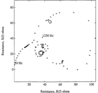
Figure 3. 113 adaptively chosen points.

[image:6.595.105.446.342.663.2]

points is also required together with an estimate of the winding angle over the entire length of the locus. Any value exceeding 180° will suffice initially since this value is re-estimated by the routine. A tolerance parameter is then required to be set before entry to the subroutine. Each subsequent call of the subroutine causes the impedance to be evaluated at the mid-point of the frequency interval. This effectively produces two sub-intervals. The chord lengths corresponding to each of the these intervals are calculated and if the angle between them is not acute or if this angle is positive (corresponding to an anti-clockwise rotation) then the subroutine is called again immediately on each of the sub-intervals. The subroutine is also called again if either the initial estimate of the winding angle (passed in the parameter list) or the new estimate of the winding angle calculated by the subroutine exceeds the given tolerance. To prevent a possibly infinite recursion when the true locus is not differentiable the subroutine is not called if the range of a frequency interval is too small. Moreover, as an extra safeguard, the subroutine is also called automatically if the range is considered to be too large.

80 ''"''"''"''"'''']'"""'''''''""'''''t''''"''"''''""''''1'"'''''''''"""''"':""""""''"''"'''t''' . . . .

60 ···:···:··· ·:····

l:Z50 Hz

40 ... ; ... " ' i " " " " " ' " " " " ' " j ' " " " ' " " " " " " " ' : " " " " ' " ' " " " " " ' ' " '

: :

. .

. .

. .

-"-""""'-....

. .

20 "" ... ; ... "" .... · ... ~ ... ! " " " " " " " ' " ' " 't"

: :

. .

. .

. .

. .

. .

. .

. .

0 .. " ... """ .... ;, .. " .... " ... : .... "" .... " .... "" ;, ""." ... ·-e.c"-'=-- ·•" " .. "" " .. " .. ".

~ ~ ;

: :

20 40 60 80 100

Resistance, R(f) ohms

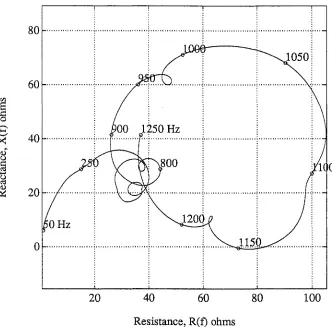
Figure 4. A parametric cubic spline on 113 points.

In practice, the user provides values for minimum and maximum frequency increments and

the algorithm effectively varies the actual increment between these bounds in a way that ultimately causes the winding angle between adjacent points to be approximately constant. The algorithm was applied to the power system locus of Figure 1, and the results are displayed

in Figure 3. It can be seen that the adaptive scheme has worked quite well on this curve. In

[image:7.597.113.446.265.593.2]

the given tolerances have prevented the algorithm from trying too hard here. A parametric cubic spline fitted through the points is displayed in Figure 4 and it cannot be distinguished by eye from the true curve of Figure 1.

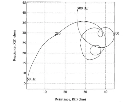
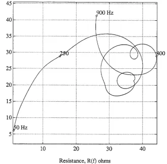
A further advantage of the adaptive scheme is seen by examining the portions of the loci

in Figures 3 and 4 corresponding to frequencies

f :::;

900. Without any further impedance

calculations, the two loci are plotted again in magnified views in Figures 5 and 6. Again there

is very little difference between these two curves, which shows that the adaptive scheme has fulfilled its task of summarising the locus well, and in a way which can withstand magnification.

45 ...

. .

00

Uz

40

··· ·· ·· ·· ··· ·r· ···· ··· ... :··· ·· ·· ·· ·· ·· .. ·· ··· ···r··· ...

~

... .

35 ... ''.' '~ ... '.' ... ' ... ;. ... '

8

30

...i::: 00

0

c

'-" 25

><

t>

(.)

[image:8.599.66.470.197.530.2]

~ ₂₀

...

(.)

~

<U

0:::

15

10 ... : ... ~ :

...

; :.

... .

5 ... ~· ... ·? ... ~ ... ·~ ... .

10 20 30 40

Resistance, R(f) ohms

Figure 5. Parametric spline on 76 adaptively chosen points.

If extra detail should be required on a sub-region, perhaps because the algorithm was initially

called with too coarse a tolerance or because the minimum increment was set too high, then it is a simple matter to apply the algorithm again with finer tolerances on each subinterval of interest without wasting any of the impedances already calculated. Thus, although it is always possible to "smooth away" loops by inappropriate choice of subroutine parameters in a first application of the algorithm, subsequent viewing of the fitted locus may suggest "filling in" some extra detail by choosing a smaller minimum increment and/ or tolerance in subsequent calls on some sub-intervals. For example, after viewing the fitted locus of Figure 4, the user

may well believe that some detail has been missed in the region around 1100 Hz.

In

fact no

essential detail has been missed in this case but confidence is easily restored by applying the algorithm again in this region to obtain a few extra impedances before replotting.

compute the parametric spline using "not-a-knot" end conditions and TGOlB to evaluate points on the fitted spline. A discussion of parametric splines, together with FORTRAN77

subroutines can be found in

[4].

45 ... : " " ' ' " ' ' ' " " " ' ' " ' ' ' ' ' ' ' : " " " " " ' ' " " " " " ' ' ' " ' : ' " ' " ' " ' ' " ' " " " " " " " ' : " " " " '

. .

. 900

fJz

.

40 • . • . . . . ' ..••... ·~' . ' ....•...•.•.••... i' ' . . . . .•...•... ~ ...••••••.•••••...•••..•..•. ~-•....•.••

; ~ : :

: :

. .

35 ··· .. ···r···r··· .... ·

: :

~

30 ₀₀

Q

' - ' 25

~

0

(.)

~

20

0

~

15

. .

[ T '.

I

: : :

: :

10 · ···r··· .. ···;···1··· ... : :

l ... ..

: :

5

... 1

...

r··· ..

1···-...

r···

: : : :

10 20 30 40

[image:9.595.129.459.128.452.2]

Resistance, R(:f) ohms

Figure 6. True locus on 851 points.

5

Conclusion

An adaptive scheme for sampling points on an impedance locus has been presented. The scheme does not depend on having a good parametrization of the locus because it is capable of adapting automatically to the local geometry of the curve. The proposed scheme is highly suited for use with parametric cubic splines to provide a smooth and accurate representation of quite complex impedance loci. Although parametric cubic splines have been used previously to represent impedance loci [6], the idea of adaptively choosing the interpolation points for the spline is new. A minor inconvenience of the proposed scheme is that the interpolation points are not calculated in order of frequency. Thus it is necessary to sort the calculated impedances before computing the cubic spline fit. This is a very small cost, however, when compared with the total calculation of all the system impedances required to produce the locus.

The work described here could be applied to any parametric curve which has the form

x

=

x(t), y

=

y(t), t

E

[t

0 ,

t

1 ], not just to impedance loci, (and also to functions,

y(x),

simply

by substituting

x(t)

=

t).

The special property of a predominantly clockwise orientation has

Finally, it is emphasised that there are many possible alternatives or refinements to the basic scheme described in Section 4. Further experience is likely to lead to improvements in future.

References

[1] Baird J., Electricity Division Audio Frequency Analysis Tool (Elafant): Programmers

Jlilan-ual, Electricity Division of the Ministry of Energy Report, 1979.

[2] Thallam R.S., Mogri S. and Burton R.S., Harmonic Impedance and Harmonic Interaction

of an AC System with lvlultiple DC lnfeeds, IEEE/PES Summer Meeting, San Francisco,

July 1987.

[3] Arrillaga J., Bradley D.A., and Badger P.S., Power System Harmonics, John Wiley &

Sons, 1985.

[4] Rice J.R, Numerical Jlilethods, Software, and Analysis, McGraw-Hill, 1983.

[5] Lahey T.L., Fortran for the 1990's, Travelling Seminar, Australia/New Zealand tour, 1989.

[6] Arrillaga J., Densem T.J., and Bodger P.S., Derivation of Power System Information at

Harmonic Frequencies, Trans. of the Institution of Professional Engineers New Zealand,