OGLE-2017-BLG-1434Lb: Eighth qqq<<<111×××101010−−−444 Mass-Ratio Microlens Planet Confirms Turnover in Planet Mass-Ratio Function
A. U d a l s k i1, Y.-H. R y u2, S. S a j a d i a n3, A. G o u l d2,4,5 and
P. M r ó z1, R. P o l e s k i1,5, M. K. S z y m a ´n s k i1, J. S k o w r on1, I. S o s z y ´n s ki1, S. K o z ł o w s k i1, P. P i e t r u k o w i c z1, K. U l a c z y k1,
M. P a w l a k1, K. R y b i c k i1, P. I w a n e k1 (OGLE Collaboration)
M. D. A l b r o w6, S.-J. C h u n g2,7, C. H a n8, K.-H. H w a n g2, Y. K. J u n g9, I.-G. S h i n9, Y. S h v a r t z v a l d10,35, J. C. Y e e9, W. Z a n g11,12, W. Z h u13, S.-M. C h a2,14, D.-J. K i m2, H.-W. K i m2,
S.-L. K i m2,7, C.-U. L e e2,7, D.-J. L e e2, Y. L e e2,14, B.-G. P a r k2,7, R. W. P o g g e5
(KMTNet Collaboration)
V. B o z z a15,16, M. D o m i n i k17, C. H e l l i n g17, M. H u n d e r t m a r k18, U. G. J ø r g e n s e n19, P. L o n g a-P e ñ a20, S. L o w r y21,
M. B u r g d o r f22, J. C a m p b e l l-W h i t e21, S. C i c e r i23, D. E v a n s24, R. F i g u e r a J a i m e s17, Y. I. F u j i i19,25, L. K. H a i k a l a26, T. H e n n i n g4, T. C. H i n s e2, L. M a n c i n i4,27,28, N. P e i x i n h o20,29,
S. R a h v a r30, M. R a b u s31,7, J. S k o t t f e l t32, C. S n o d g r a s s33, J. S o u t h w o r t h24, C. v o n E s s e n34
(MiNDSTEp Collaboration)
1Warsaw University Observatory, Al. Ujazdowskie 4, 00-478 Warszawa, Poland email: [email protected]
2Korea Astronomy and Space Science Institute, Daejon 34055, Korea 3Department of Physics, Isfahan University of Technology, Isfahan 84156-83111, Iran
4Max-Planck-Institute for Astronomy, Königstuhl 17, 69117 Heidelberg, Germany 5Department of Astronomy, Ohio State University, 140 W. 18th Ave., Columbus,
OH 43210, USA
6University of Canterbury, Department of Physics and Astronomy, Private Bag 4800, Christchurch 8020, New Zealand
7Korea University of Science and Technology, Daejeon 34113, Korea 8Department of Physics, Chungbuk National University, Cheongju 28644,
Republic of Korea
9Harvard-Smithsonian CfA, 60 Garden St., Cambridge, MA 02138, USA 10Jet Propulsion Laboratory, California Institute of Technology, 4800 Oak Grove Drive,
Pasadena, CA 91109, USA
12Department of Physics, Zhejiang University, Hangzhou, 310058, China 13Canadian Institute for Theoretical Astrophysics, University of Toronto,
60 St George Street, Toronto, ON M5S 3H8, Canada
14School of Space Research, Kyung Hee University, Yongin, Kyeonggi 17104, Korea 15Dipartimento di Fisica "E.R. Caianiello", Università di Salerno,
Via Giovanni Paolo II 132, 84084, Fisciano, Italy
16Istituto Nazionale di Fisica Nucleare, Sezione di Napoli, Napoli, Italy 17Centre for Exoplanet Science, SUPA, School of Physics & Astronomy, University of St Andrews, North Haugh, St Andrews KY16 9SS, UK
18Astronomisches Rechen-Institut, Zentrum für Astronomie der Universität Heidelberg (ZAH), 69120 Heidelberg, Germany
19Niels Bohr Institute & Centre for Star and Planet Formation, University of Copenhagen, Øster Voldgade 5, 1350 Copenhagen, Denmark
20Unidad de Astronomía, Universidad de Antofagasta, Av. Angamos 601, Antofagasta, Chile
21Centre for Astrophysics & Planetary Science, The University of Kent, Canterbury CT2 7NH, UK
22Universität Hamburg, Faculty of Mathematics, Informatics and Natural Sciences, Department of Earth Sciences, Meteorological Institute, Bundesstraße 55,
20146 Hamburg, Germany
23Department of Astronomy, Stockholm University, Alba Nova University Center, 106 91, Stockholm, Sweden
24Astrophysics Group, Keele University, Staffordshire, ST5 5BG, UK
25Institute for Advanced Research, Nagoya University, Furo-cho, Chikusa-ku, Nagoya, 464-8601, Japan
26Instituto de Astronomia y Ciencias Planetarias de Atacama, Universidad de Atacama, Copayapu 485, Copiapo, Chile
27Department of Physics, University of Rome Tor Vergata, Via della Ricerca Scientifica 1, I-00133-Roma, Italy 28INAF – Astrophysical Observatory of Turin, Via Osservatorio 20,
I-10025 – Pino Torinese, Italy
29CITEUC – Center for Earth and Space Research of the University of Coimbra, Geophysical and Astronomical Observatory, R. Observatorio s/n, 3040-004 Coimbra,
Portugal
30Department of Physics, Sharif University of Technology, PO Box 11155-9161 Tehran, Iran
31Instituto de Astrofísica, Pontificia Universidad Católica de Chile, Av. Vicuña Mackenna 4860, 7820436 Macul, Santiago, Chile
32Centre for Electronic Imaging, Department of Physical Sciences, The Open University, Milton Keynes, MK7 6AA, UK
33School of Physical Sciences, Faculty of Science, Technology, Engineering and Mathematics, The Open University, Walton Hall, Milton Keynes, MK7 6AA, UK 34Stellar Astrophysics Centre, Department of Physics and Astronomy, Aarhus University,
Ny Munkegade 120, 8000 Aarhus C, Denmark 35NASA Postdoctoral Program Fellow
ABSTRACT
We report the discovery of a cold Super-Earth planet ( mp=4.4±0.5 M⊕) orbiting a
low-mass ( M=0.23±0.03 M⊙) M dwarf at projected separation a⊥=1.18±0.10 a.u., i.e., about 1.9 times the distance the snow line. The system is quite nearby for a microlensing planet, DL= 0.86±0.09 kpc. Indeed, it was the large lens-source relative parallax πrel=1.0 mas (combined
with the low mass M ) that gave rise to the large, and thus well-measured, “microlens parallax”
πE∝(πrel/M)1/2 that enabled these precise measurements. OGLE-2017-BLG-1434Lb is the eighth
microlensing planet with planet-host mass ratio q<1×10⁻⁴.
We apply a new planet-detection sensitivity method, which is a variant of “V/Vmax”, to seven
of these eight planets to derive the mass-ratio function in this regime. We find dN/d ln q∝qp, with
p=1.05+−00..7868, which confirms the “turnover” in the mass function found by Suzuki et al. relative to the power law of opposite sign n=−0.93±0.13 at higher mass ratios q&2×10⁻⁴. We combine
our result with that of Suzuki et al. to obtain p=0.73+−00..4234.
Key words: Gravitational lensing: micro – Planetary systems
1. Introduction
Microlensing searches are finding planets with planet/host mass ratio q that
are nearly uniformly distributed in log q over −4.3.log q.−2 (Figs. 7 and
8 of Mróz et al. 2017). Since planet detectability grows with q , this immedi-ately implies a steeply rising mass function toward lower mass ratios. In the first
study to measure this relation, Sumi et al. (2010) found dN/d log q∝qn with
n=−0.7±0.2 . Naively, the almost perfectly flat distribution cataloged by Mróz
et al. (2017) over a 2.3 dex range in q would indeed appear to argue for a single
power law. However, Suzuki et al. (2016) subsequently argued for a break in the
power law at about log q≈ −3.75 , with n=−0.93±0.13 above the break.
Be-low the break they found a sign reversal in the power law, dN/d log q∝qp with
p=0.6+0−0..54, implying a true “turnover” at the break. The main argument for this
break is that existing planet surveys had significant sensitivity to planets below the break, but found very few. In particular, the Microlensing Observations in Astro-physics (MOA) survey, which was the primary data set that they analyzed, had only
two planets with log q<−4 (or four in extended sample). Note, however, that
an-other recent study by Shvartzvald et al. (2016), based on the overlap of the OGLE,
MOA and Wise surveys, fit to a single power law and found n=−0.50±0.17 .
A confirmation and refined measurement (or, alternatively, refutation) of the Suzuki et al. (2016) break and turnover would be of great interest to constrain theories of planetary formation. Moreover, it would also be of immediate practical interest in devising strategies for WFIRST microlensing observations (Spergel et
al. 2013). Since WFIRST will be far more sensitive to planets below the Suzuki et al. (2016) break than ground-based surveys, its planet discovery rate is much more
sensitive to such a break.
Here, we report the discovery of the low mass ratio q=5.8×10⁻⁵ planet
OGLE-2017-BLG-1434Lb. This is the eighth microlensing planet with a mass
below the Suzuki et al. (2016) break is now large enough for robust statistical in-vestigation. On the other hand, in contrast to the Suzuki et al. (2016) sample, these eight planets are drawn from quite heterogeneous detection processes. Therefore proper statistical analysis requires great care.
There are two other notable features of the discovery of OGLE-2017-BLG-1434Lb. First, we are able to make an accurate mass measurement, thanks to a clear detection of the microlens parallax parameter,
πππE≡πE
µµµrel µrel
, πE≡
πrel
θE
(1)
where πrel≡a.u.(DL−1−D−S1) and µµµrel are the lens-source relative parallax and
proper motion, respectively,
θE≡√κMπrel, κ≡
4G
c2a.u.≃8.14 mas
M⊙, (2)
and M is the lens mass. Note that whenπE andθEare both measured, M=θE/κπE
can likewise be determined (Gould 1992, 2000, 2004, Gould and Horne 2013)
Of the eight planets with log q<−4 , five have good-to-excellent mass
mea-surements, which is a remarkably high fraction. Two of these (including OGLE-2017-BLG-1434) have excellent ground-based parallax measurements, one has a good ground-based parallax measurement, one has an excellent space-based par-allax measurement using Spitzer satellite, and for the last, the host was directly imaged 8.2 years after the event. This high rate of mass measurements permits at least a qualitative statement about the distribution of host masses of low mass-ratio planets.
Second, although OGLE-2017-BLG-1434 is within a factor 1.3 of the lowest mass-ratio microlensing planet, we show that it would have been both detected and
well-characterized even if it were a factor 30 smaller in q , i.e., log q=−5.71 , or
approximately 12 Moon masses. This demonstrates that microlensing studies, at least in their current configuration, can probe to substantially smaller masses than have yet been reported as discoveries, and hence further motivates an investigation
of whether there is really a break in the mass-ratio function near log q≈ −4 .
2. Observations
OGLE-2017-BLG-1434 is at (RA,Dec)J2000 = (17:53:07.29,−30 :14:44.6),
cor-responding to (l,b) = (−0.28,−2.07). It was discovered and announced as a
probable microlensing event by the OGLE Early Warning System (Udalski et al.
1994, Udalski 2003) at UT 19:33 July 25, 20171. The event lies in OGLE field
1The same microlensing event triggered an alert (OGLE-2017-BLG-1392) on a different catalog
BLG501 (Udalski et al. 2015), for which OGLE observations were at a cadence
of Γ=1 hr−1 during the 2017 season using their 1.3 m Warsaw telescope at Las
Campanas, Chile.
The Korea Microlensing Telescope Network (KMTNet, Kim et al. 2016) ob-served this field from its three 1.6 m telescopes at CTIO (Chile, KMTC), SAAO (South Africa, KMTS) and SSO (Australia, KMTA), in its two slightly offset fields
BLG01 and BLG41, with combined cadence of Γ=4 hr−1 .
The great majority of these survey observations were carried out in I-band with occasional V-band observations made solely to determine source colors. All reduc-tions for the light curve analysis were conducted using variants of difference image analysis (DIA, Alard and Lupton 1998), specifically Wo´zniak (2000) and Albrow
et al. (2009).
The MiNDSTEp collaboration observed OGLE-2017-BLG-1434 from the 1.54 m Danish Telescope at La Silla, Chile, using an EMCCD camera operated at 10 Hz and with a broad passband approximating the I-band filter, with mean response at 770 nm (Skottfelt et al. 2015, Evans et al. 2016). The data were reduced using an updated version of the DanDIA pipeline (Bramich 2008). These observations were
initiated with 10 exposures on the night of HJD′≡HJD−2 450 000=7981 and
continually increased to 75 exposures on HJD′=7984 , i.e., the night closest to the
predicted peak, falling to 50 exposures the following night. Based on these last observations, MiNDSTEp issued an alert, triggered by SIGNALMEN (Dominik et
al. 2007), of a possible anomaly, which it confirmed the next day based on OGLE
online data. MiNDSTEp then continued regular observations of the event until the
night of HJD′=7998 .
3. Analysis
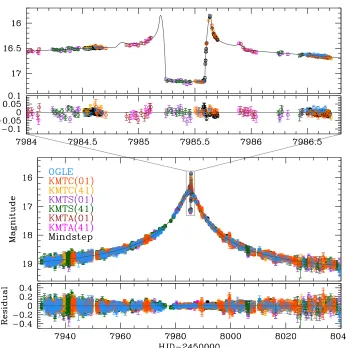
With the exception of some deviations near the peak that last slightly more than one day, the overall shape of the OGLE-2017-BLG-1434 light curve (Fig. 1) is that of an ordinary point-lens (Paczy´nski 1986) event. Excluding the deviation, the
change in magnitude from baseline to peak (≈2.5 mag) implies a magnification
A&10 (higher if there is significant blending). The two most obvious components of the deviation are a flat trough that lies about 0.7 mag below the level of the point-lens curve and lasts 0.4 d (traced in KMTS, OGLE, KMTC, and MiNDSTEp data), followed by a very rapid caustic entrance (traced in KMTC, OGLE, and MiND-STEp data). Once these features are noted, it becomes clear that the underlying light curve is essentially symmetric and that the onset of a caustic exit is traced by KMTA data just before the trough.
Fig. 1. Light curve and best-fit model of OGLE-2017-BLG-1434. As discussed in Section 3, many of the key parameters can be “read off” the light curve, including that this is a very low mass-ratio planet: q<10−4. Data are color-coded by observatory.
two images is η= (A−1)/(A+1) where A is the total magnification. Hence, for
a high-magnification event such as this one, η→1 , which means that annihilating
the minor image should decrease the total flux by half, i.e.,≈0.75 mag. That is,
the light curve’s behavior exactly corresponds to this expectation.
Such troughs are always aligned with the planet-star axis and are flanked by two caustics. However, the troughs generally extend substantially beyond the caustics. Hence, if the source trajectory crosses the trough at a point where there are no caustics, its entrance and exit to the trough will be smooth. However, if it crosses the caustics, the trough entrance and exit will correspond to a sharp (discontinuous slope) caustic exit and entrance, respectively. The latter is clearly the geometry of OGLE-2017-BLG-1434.
than its “outer walls”, the effect on the light curve is much less pronounced. Never-theless, this outer-edge crossing was captured in the first three KMTA points after the trough.
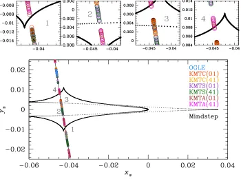
[image:7.612.111.461.238.498.2]If the trough occurs at relatively low magnification, then each of the two caustic “walls” that flank the caustic will be part of triangular caustic structures. However, at progressively higher magnification (corresponding to planets that are progres-sively closer to the Einstein ring), these triangular caustics grow in size and pro-gressively move toward the quadrilateral central caustic close to the host. The trian-gular caustics eventually merge with the central caustic to form a single, six-sided caustic (Fig. 4 of Gaudi 2012). This turns out to be the geometry of OGLE-2017-BLG-1434. See Fig. 2.
Fig. 2. Caustic diagram of OGLE-2017-BLG-1434. The source passes over the “planetary wing” of a resonant caustic, resulting from the planet perturbing the minor image. The points are color coded by observatory, and their size represents the scaled sourceρ=4.5×10⁻⁴ of the best fit model.
Continuing this logic, one can approximately read off the parameters of a stan-dard seven-parameter model from the light curve, using known analytic formula
(Han 2006) for the caustics. Three of these parameters(t0,u0,tE)correspond to the
time of maximum, impact parameter, and Einstein crossing time of the underlying
point-lens (Paczy´nski 1986) model. Three others(s,q,α) describe the binary
com-panion, namely its separation (in units of θE), its mass ratio, and the angle of the
source passes over or near the caustics, one must specifyρ=θ∗/θE, i.e., the ratio of the source radius to the Einstein radius.
A point-lens fit to the light curve with the anomaly removed yields (t0,u0,tE) =
(7984.94,0.027,95 d), which implies an effective timescale teff≡u0tE=2.57 d.
The anomaly is centeredδt=0.5 d after peak, implying thatα=atan(−teff/δt) =
±259◦ and that s should satisfy, s−1−s =u0
p
1+ (δt/teff)2, which implies2
s≃1−u0/2=0.986 . From the light curve, the duration of the trough is∆t≃0.4 d.
(It could in principle be slightly larger because the caustic exit is not actually ob-served. However, the rise toward the caustic is observed from KMTA, so this estimate cannot be far off.) This quantity can be related to the Han (2006)
pa-rameter ηc− =2q1/2(s−2−1)1/2 by ∆t=2tEηc−|secα|, which for the present
case implies q≃u0(∆t/teff)2/16=4.1×10−5. Finally, the rise time of the
caus-tic exit in OGLE/KMTC/MiNDSTEp data is trise =66 min. From Gould and
Andronov (1999), trise =1.7t∗secα, where t∗ =ρtE. Hence, t∗ =39 min and
ρ≃(t∗/tE) =3.5×10⁻⁴.
However, following from these results, it is obvious that additional higher order
effects should be measurable. First note that ρ is unusually small, so that the
Einstein radiusθE=θ∗/ρ≃3000θ∗. We will estimate the source size θ∗ in detail
in Section 4.1. However, just from the source flux derived from the Paczy´nski
(1986) fit, it is an upper main sequence star, i.e.,θ∗∼0.5 µ as.
Such a large Einstein radius (θE≈1.5 µ as) immediately implies that the host
must be either a dark remnant (black hole or neutron star) or it must be quite nearby.
That is, from the definition ofθE (Eq. 2),
πrel=
θ2
E
κM →0.3 µas
M
M⊙
−1
. (3)
Indeed, since a solar-mass star at DL≈2.5 kpc would easily be visible, the actual
lens must have even lower mass (hence higher πrel). Therefore, again unless the
host is a dark remnant, the microlens parallax must be fairly large.
πE=
πrel
θE
>0.2. (4)
Given that the event is quite long, such a parallax should be measurable.
Thus, without any detailed modeling, one can infer that there should be a strong microlens parallax signal and that the implications of not finding such a signal would be striking.
When introducing the two parallax parameters πππE = (πE,N,πE,E), one must
also, at least initially, introduce linearized orbital motion parameters(ds/dt,dα/dt)
as well. These encode the instantaneous rate of change in the separation and
ori-entation of the binary at t0. There are two reasons that these must be included.
First, the orbital motion parameters (ds/dt,dα/dt) can be correlated withπππE, so
that by ignoring them one can induce artificial effects in the parallax (Skowron et
al. 2011, Batista et al. 2011, Han et al. 2016). Second, binary systems are known a priori to orbit their center of mass. Hence, there is no viable reason for
exclud-ing these parameters except if they are better constrained by the fact that physical systems ought to be bound than they are by the data. However, while (as described above) there are very strong reasons to believe that the parallax parameters can be
measured, there is no corresponding confidence with respect to (ds/dt,dα/dt).
Therefore, these parameters must be handled carefully. See, e.g., Ryu et al. (2017). Notwithstanding the above analytic arguments, we conduct a grid search over
(s,q,α), seeded by the above values of (t0,u0,tE,ρ), with all parameters except
(s,q) allowed to vary and apply χ2 minimization using a Markov Chain Monte
Carlo (MCMC). To evaluate the magnifications at individual data points, we use inverse ray shooting in and near the caustics (Kayser et al. 1986, Schneider and Weiss 1988, Wambsganss 1997) and multipole approximations (Pejcha and Hey-rovský 2009, Gould 2008) elsewhere. We employ a linear limb-darkening
coeffi-cientΓI=0.429 based on the source type derived in Section 4.1.
We find only one solution. This is close to the one derived above
analyt-ically in terms of (s,α) and the so-called invariant quantities (Yee et al. 2012,
Ryu et al. 2017): (s,α,teff,t∗,qtE) = [0.981,259◦,(2.59,0.0284,0.00364)d]
com-pared to[0.986,259◦,(2.57,0.0271,0.00389)d]“predicted”. The major difference
is only in tE, which can be significantly impacted by unmodeled parallax for long
timescale events.
We then introduce the higher-order parameters πππE = (πE,N,πE,E) and
γγγ= ((ds/dt)/s,dα/dt). We find that in a completely free fit, three of these are
well constrained, but the fourth(γ⊥=dα/dt) is not. In particular, we find that for
most of the solution space, the (absolute value of the) ratio of projected kinetic to potential energy (Batista et al. 2011),
β≡ KE PE ⊥
= κM⊙yr 2
8π2
πE
θE
s3γ2
(πE+πs/θE)3
, (5)
violates the boundedness condition,β<1 . Here, we adoptπs=0.117 mas for the
source parallax. We address this by making two different calculations. First, we
arbitrarily set γγγ=0 . Of course, as mentioned above, this is unphysical, but it is
simple and is useful as a benchmark for the second calculation, in which we allowγγγ
to vary but restrictβ<0.7 , i.e., a limit that would be satisfied by the overwhelming
majority of real, bound systems3.
The results are shown in Table 1. The first point is that the parallax+orbital
models in whichβ is restricted to a reasonable physical rangeβ<0.7 yield
statis-tically indistinguishable results from the parallax-only models in whichβ=γ=0 .
That is, our inability to fully measure γ does not significantly influence the
mea-surement of any other parameter.
Second, while there are two degenerate (±u0) models with similar χ2, their
parameters (apart from the sign of u0) are the same within 1σ. Hence, this
degen-eracy does not materially impact the inferred physical parameters of the system.
T a b l e 1
Best-fit solutions
Parallax models Parallax+Orbital motion models
Parameters Standard u0>0 u0<0 u0>0 u0<0
χ2/dof 21418.644/18659 18658.511/18657 18662.277/18657 18654.143/18655 18658.155/18655
t0[HJD’] 7984.935±0.004 7984.979±0.004 7984.978±0.004 7984.978±0.004 7984.977±0.004
u0 0.037±0.001 0.044±0.001 −0.044±0.001 0.043±0.001 −0.043±0.001
tE[d] 72.856±0.907 61.421±0.692 62.981±0.788 62.957±0.863 64.255±1.006
s 0.980±0.0003 0.978±0.0003 0.978±0.0003 0.979±0.0004 0.979±0.0003
q(10−5) 4.938±0.057 5.866±0.063 5.571±0.077 5.722±0.145 5.607±0.152
α[rad] 4.535±0.001 4.552±0.001 −4.556±0.002 4.551±0.002 −4.553±0.002 ρ(10−4) 4.019±0.060 4.815±0.068 4.679±0.072 4.692±0.093 4.643±0.099 πE,N − −0.491±0.079 −0.508±0.083 −0.586±0.081 −0.562±0.081
πE,E − 0.471±0.013 0.475±0.013 0.472±0.013 0.471±0.013
ds/dt[yr−1] − − − 0.069±0.044 0.090±0.044
dα/dt [yr−1] − − − −0.218±1.432 −1.543±1.459
fS 0.139±0.002 0.167±0.002 0.166±0.002 0.162±0.003 0.163±0.003
fB 0.193±0.002 0.165±0.002 0.166±0.002 0.170±0.003 0.169±0.003
The fluxes fS and fB are normalized to I=18 mag in OGLE-IV instrumental magnitude scale, or Istd=
18.085 mag in calibrated I-band magnitudes.
In the “Parallax+Orbital” models, the parameterβ≡(KE/PE)⊥is restricted toβ<0.7. See text.
4. Physical Parameters
4.1. Measurement of θE and µ
We derive the source brightness from the model presented in Section 3 and derive the color from regression. We then find the offset from the clump on an
instrumen-tal color–magnitude diagram: [(V−I),I]s−[(V−I),I]clump= (−0.328,+3.990)±
(0.023,0.038). We adopt[(V−I),I]clump= (1.06,14.46)from Bensby et al. (2013)
and Nataf et al. (2013), respectively, and so derive[(V−I),I]s= (0.732,18.45)±
(0.025,0.063). We convert from V/I to V/K using the VIK color–color relations
of Bessell and Brett (1988) and finally derive
θ∗=0.657±0.041 µas (6)
using the color/surface-brightness relations of Kervella et al. (2004). Incorporating parameters from Table 1, we thereby derive.
θE=
θ∗
ρ =1.40±0.09 mas, µ=
θ∗
tE
4.2. Masses, Distance, and Projected Separation
Combining the results of Section 4.1 and Table 1, we find
M= θE
κπE
=0.234±0.026 M⊙ mp=
q
1+qM=4.4±0.5 M⊕ (8)
DL=
a.u.
θEπE+πs
=0.86±0.09 kpc a⊥=sθEDL=1.18±0.10 a.u. (9)
where we have adopted a source parallaxπs=0.117±0.010 mas and where a⊥ is
the projected separation. That is, the planet is a super-Earth orbiting a middle-late M dwarf. If we adopt a “snow line” scaled to host mass (e.g., Kennedy and Kenyon
2008), and anchored in the observed Solar-system value, asnow=2.7 a.u.(M/M⊙),
then this planet lies projected at a⊥=1.9 asnow.
5. Microlensing Earths and Super-Earths with Well-Measured Masses
OGLE-2017-BLG-1434Lb joins a small list of Earths and Super-Earths with well-measured masses discovered by microlensing. To be an “Earth or
Super-Earth”, we require a best-estimated planet mass mp<7 M⊕. To be “well-measured”
we set two requirements. First we require that the quoted 1σ error on the planet
mass measurement span a factor <2 , i.e.,σ(log mp)<0.15 . Second, we require
that the host mass was determined either by measuring both πE and θE (as was
done here) or by directly imaging the host.
We review the literature (effectively updating the summary by Mróz et al. 2017) and find only three such planets: OGLE-2016-BLG-1195Lb (Bond et al. 2017, Shvartzvald et al. 2017), OGLE-2013-BLG-0341LBb (Gould et al. 2014) and OGLE-2017-BLG-1434Lb (this work). In all cases, the mass determination
is via measurements of θE and πE. We note that there is another planet,
MOA-2007-BLG-192Lb (Bennett et al. 2008, Kubas et al. 2012) whose host mass was quite well determined by direct imaging and whose best-estimated planet mass
mp=3.2+5−1..28 falls in the defined range. However, the error bars on the planet
[image:11.612.126.448.565.622.2]mass are far too large to meet our criterion.
Table 2 gives the main characteristics of these systems.
T a b l e 2
Characteristics of Earth/Super-Earth Events
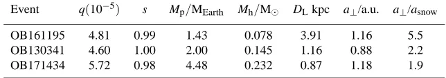
Event q(10−5) s Mp/MEarth Mh/M⊙ DLkpc a⊥/a.u. a⊥/asnow
OB161195 4.81 0.99 1.43 0.078 3.91 1.16 5.5 OB130341 4.60 1.00 2.00 0.145 1.16 0.88 2.2 OB171434 5.72 0.98 4.48 0.232 0.87 1.18 1.9
The first point to note about these three well-constrained low-mass planets is that they all have low-mass hosts, i.e., from the hydrogen-burning limit to a middle-late M dwarf. The second point is that all are seen projected close to the Einstein
ring, s≈1 . And the third is that two of the three are extremely nearby, DL.1 kpc.
All three of these characteristics are heavily influenced by selection, but none can be regarded purely as a selection effect.
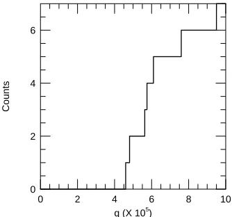
As illustrated by Fig. 3, there are no microlensing planets with q.5×10−5.
This fact, combined with our sample requirement mp<7 M⊕, already implies
that the hosts will be M.0.4 M⊙. However, as we will show in Section 6, the
apparent “barrier” at q≈5×10⁻⁵ is not a selection effect: lower mass ratios could
have been detected if such planets were common.
q (X 105 )
Counts
0 2 4 6 8 10
[image:12.612.207.374.229.385.2]0 2 4 6
Fig. 3. Cumulative distribution of planet/host mass ratios q for the seven microlens planets with well-defined measurements q<10−4. Five of the seven have 4.6×10⁻⁵≤q≤6.1×10⁻⁵, suggesting either a rapid drop either in sensitivity of microlensing experiments to low mass-ratio planets or in the frequency of such planets.
Similarly, it is well-known that it is easier to detect planets when they lie pro-jected close to the Einstein ring. In particular, for relatively high-magnification events, which applies to all three of these planets, planet-sensitivity diagrams have
a triangular shape that is symmetric about log s=0 (Gould et al. 2010). However,
since (as just mentioned) planets could have been detected at lower q , it follows
immediately that they could also have been detected at higher |log s|.
Finally, ground-based parallax measurements are heavily biased toward nearby
lenses, simply because the microlens parallax is larger: πE= (πrel/κM)1/2.
6. Planet Mass-Ratio Function at the Low-Mass End
At q=5.8×10⁻⁵, OGLE-2017-BLG-1434Lb is the eighth published
microlens-ing planet with a planet/host mass-ratio measurement that places it securely in the
[image:13.612.233.342.278.333.2]range q<10−4. Strikingly, these are mostly clustered close to q≈5×10⁻⁵. See
Fig. 3. This would seem to indicate a sharp cutoff either in sensitivity or in the exis-tence of planetary companions at the separation ranges accessible to microlensing. Because the discovery process of these planets is quite heterogeneous, it is not possible to reliably determine an absolute mass-ratio function from this sample. That is, there is no way to estimate the rate of non-detections from which this sample was drawn.
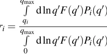
However, by applying the technique of “V/Vmax” (Schmidt 1968), we can use
this sample to constrain the relative frequency by mass ratio. That is, we can
con-sider various trial mass-ratio functions F(q). For each detected planet i , we
evalu-ate the “V/Vmax” ratio ri defined by
ri= qmax
R
qi
d ln q′F(q′)Pi(q′)
qmax R
0
d ln q′F(q′)Pi(q′)
(10)
where qmax=10−4 (i.e., the definition of the sample) and Pi(q′) is the probability
that the planet would have been detected and published if the event had had exactly
the same parameters as the actual one, but with a different q′6=qi.
If F(q) has been chosen correctly, then the distribution of the ri should be
consistent with being drawn from a uniform distribution over the interval [0,1].
Hence, all trial mass-ratio functions F(q) that yield a distribution of ri that is
inconsistent with uniform can be ruled out.
In principle, one might consider each Pi to be a continuous function varying
between zero and one. For example, one might decide that P3(q′=1.3×10⁻⁵) =
43% . That is, the light curve associated with the third event (and with the specified
q′) would have had a 43% chance of having been noticed as planetary in nature and
then generating sufficient confidence in the evaluation to publish it. In fact, we will
approximate the Pi(q) as bi-modal, either 0 or 1. In most cases, this means that
there is some continuous interval over which the planet is judged to be detectable,
defined by qmin,i. Then Eq.(10) would become
ri→ qmax
R
qi
d ln q′F(q′)
qmax R
qmin,i
d ln q′F(q′)
. (11)
6.1. Evaluation of qmin,i and Pi(q′)
We define our sample by the following three criteria:
(1) Best-fit mass ratio log q<−4 ,
(2) Formal error estimateσ(log q)<0.15 ,
(3) No alternate solutions with∆χ2<10 and∆log q>0.3 .
Criterion (1) is the regime that we seek to probe. Planetary candidates that fail criterion (2) generally cannot be securely identified as being in the sample. Moreover, for planets with larger error bars, there is an increasing (and basically unknowable) probability that they would not be published. Candidates that fail
criterion (3) are ambiguous in the sense that qmin can be substantially different for
different solutions.
For consistency with these choices, we likewise set Pi(q′) =0 for any choice
of q′ that leads to failure of either criterion (2) or (3).
We find that one of the eight planets that satisfy criteria (1) and (2), fails cri-terion (3): OGLE-2017-BLG-0173 (Hwang et al. 2018). In fact, at the time that we devised these criteria, it was not yet known that OGLE-2017-BLG-0173 suf-fered from such a degeneracy. More generally, we did not alter our criteria as we studied the eight planets in detail. Even though one of these, OGLE-2017-BLG-0173, will be excluded from the sample, we include it in this part of the analysis for completeness and to explore the problems posed by this type of degeneracy.
Here we evaluate the range of q over which each of the eight planets that satisfy criteria (1) and (2) would have been detected. In each case we discuss the methods by which the planet was detected, or could have been detected using approaches that were applied to essentially all events in its class. “Detection” here requires that a simulated planet must meet two criteria: first, that it would have been noticed as a potential planet based on whatever data were routinely available, and second, that further analysis based on re-reduced data (plus whatever archival data would have been available) would have led to an unambiguous planet, worthy of publication. Because all the planets discussed here have low mass ratio q , we assume that if the planet was publishable, it would in fact have been published. (This is not actually true for some higher mass-ratio planets, which sometimes take many years to elicit enough enthusiasm to push through to publication.)
OGLE-2017-BLG-1434
As we show below, at sufficiently low q , there would have been no noticeable deviations as seen from Chile, but there would still have remained significant devi-ations as seen from South Africa. In these limiting cases, there would have been no MiNDSTEp alert. The path to anomaly recognition would then have been the reg-ular KMTNet review of ongoing events. This review would have combined OGLE online data with KMTNet “quick look” data. Hence, this is what we simulate be-low.
Fig. 4 shows the anomalous region of the light curve in on-line OGLE data and quick-look KMTNet data as it would have appeared with exactly the same parameters shown in Table 1, except with q taking on other values. To construct this figure, we measure the residuals from the best-fit model for each data point and
renormalize the errors (with uniform error rescaling) so that χ2/do f =1 . Then
for each observatory, we create a fake light curve whose value is the model light curve plus the residual in magnitudes, and whose error bar is the same as that of the original (renormalized) data point. In each case, we show both the original model and the model with different q that was used to construct the fake light curves. Note that the KMTNet “quick look” data consisted only of observations from field BLG41 (and not BLG01) and so are at half the cadence of the final KMTNet data that are shown in Fig. 1.
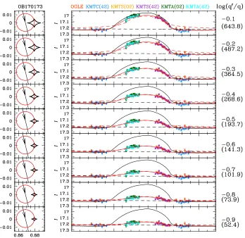
Fig. 4 has nine panels corresponding to log(q′/q) =−0.25,−0.5, . . .−2.25 .
Careful inspection of the log(q′/q) =−1.75 panel shows clear systematic
resid-uals, with two consecutive points below the point-lens curve, with the lower one
being below by≈0.3 mag. However, a cursory inspection would have shown only
a single clearly outlying point. Based on the direct experience of the KMTNet team, we consider that it is possible that these would have triggered a further investiga-tion, i.e., first corroboration in the BLG01 data and, following this, re-reduction of all of the data. However, we judge that the probability for this is substantially below 50%, and hence within the framework we have adopted, we approximate this
proba-bility as P=0 . By contrast, the “quick look” data for log(q′/q) =−1.50 , with two
points well below the single-lens curve, and one of them by≈0.6 mag would
cer-tainly have triggered such an investigation. On the other hand, log(q′/q) =−2.0
would certainly not have triggered such an investigation, but even it had, the re-reduced data would not have yielded a publishable detection because the signal is too weak.
To assess publishability, we first consider the marginally recognizable case,
log(q′/q) =−1.75 . We model the fake re-reduced data in exactly the same way
that we modeled the real data except that we exclude orbital motion (which would not be measurable for such a short and weak anomaly, and also would not be at all required for publication). We find that the planet’s parameters in this case are
well constrained, for example log q=−5.88±0.072 . This error bar is well within
the limit set by criterion (2). We note that the best fit value (−5.88 ) differs by
re-Fig. 4. Nine simulations of OGLE-2017-BLG-1434 with exactly the same parameters as the best-fit model (black curve) except that the mass ratio q is lower by ∆log q as indicated in the right axis labels. In each case, the simulated data points (various colors) deviate from the model (orange curve) by exactly the same amount as the actual data points deviate from the best-fit model. The left panels show the corresponding caustic geometries. These characteristics will be same for all eight events in the figures that follow. The data points are based on the “online” OGLE data and “quick look” KMTNet data in order to focus on the problem of determining whether the event would be recognized as sufficiently interesting to trigger re-reductions.
flects the fact that the residuals, which concretely reflect the observational errors, are preserved in the simulated data. It follows that the much stronger signal at
log(q′/q) =−1.50 would also meet our criteria. We therefore adopt this threshold.
Before continuing, we note that more systematic procedures are currently be-ing applied to 2017 KMTNet data, by means of which it is very likely that at
log(q′/q) =−1.75 , this planet would ultimately have been discovered. That is,
(whether discovered by KMTNet or others) will by mid-2018 be reviewed using all available KMTNet data. However, such “ultimate discoveries” are irrelevant to the analysis being conducted here. All real planets that will “ultimately be discovered” are presently unknown, and thus are automatically excluded. Therefore, we must equally exclude simulated planetary events in this class.
OGLE-2017-BLG-0173
Hwang et al. (2018) analyzed OGLE and KMTNet data for OGLE-2017-BLG-0173 and found three solutions, including two “von Schlieffen” solutions (A,C)
with q≈6.5±0.9×10⁻⁵, and one “Cannae” solution (B) with q≈2.5±0.2×
10−5. All three solutions have s≈1.5 . Two of these solutions (A,B) differ by
only ∆χ2=3.5 , so this planet fails criterion (3), even though it satisfies criteria
(1) and (2). Hence, this planet is excluded from our sample. Nevertheless, as
mentioned above, we analyze it for completeness. Since solution (C) has∆χ2=16 ,
we focus here on solutions (A,B).
As shown in their Fig. 1, the event betrays no hint of an anomaly in OGLE data, so the decision to examine quick-look KMTNet data was not influenced in any way by the presence of a planet. Thus, we must evaluate the minimum value of q that would have triggered a decision to re-reduce the data and then determine whether the resulting light curve would have been reliable enough to warrant publication of the (putative) planet. We note that, as shown in their Fig. 3, the “bump” in the KMTNet data was caused by the edge of a large source grazing the center of the caustic for solution (A) and by the center of a large source passing directly over the caustic for solution (B). Figs. 5 and 6 show sets of nine simulated light
curves for log(q′/q) =−0.1,−0.2, . . .−0.9 , for solutions A and B, respectively.
The first point is that to the eye, the two figures look identical, except that the geometries at the left are quite distinct. Second, one sees that within each figure, the bump looks qualitatively similar in all cases, which is fundamentally due to the “Hollywood” (Gould 1997, Hwang et al. 2018) character of the event. The
main difference is that the height of the bump scales ∝q (as discussed by Hwang
et al. 2018 see their Eqs.(9) and (10)). We estimate that at log(q′/q) =−0.7 the “bump” (now 0.06 mag, compared to the actual one of 0.3 mag), would have still triggered a further investigation for either solution A or B. Further, the numbers
at the right show∆χ2=χ2(1L2S)−χ2(2L1S) between binary-source (1L2S) and
binary-lens (2L1S) models. These values are certainly high enough to exclude the 1L2S interpretation.
However, we find that at log(q′/q) =−0.7 , and indeed at all q′ shown in the
figures, the analysis of either simulated data set (A or B) yields a discrete
degener-acy between the two classes of models (von Schlieffen and Cannae), with∆χ2<10
and∆log q>0.3 between the two minima. That is, they all suffer from essentially
the same degeneracy as the original event. Hence, although for log(q′/q)≥ −0.7 ,
Fig. 5. Nine simulations of OGLE-2017-BLG-0173 (von Schlieffen solution A), similar to Fig. 4. The values in parentheses are ∆χ2=χ2(1L2S)−χ2(2L1S), by which binary source models are
excluded. To the eye, the degeneracy between these solutions and those in Fig. 6 (Cannae solution B) persists at all q .
This exclusion has no practical importance from the perspective of the present mass-ratio-function analysis, because the original event is itself excluded. How-ever, the persistence of this degeneracy is of significant interest. Hwang et al. (2018) had noted that the other published Hollywood event, OGLE-2005-BLG-390 (Beaulieu et al. 2006), did not suffer from this von Schlieffen/Cannae degeneracy. And they further noted that the caustic was much smaller than the source in that case, whereas the caustic was of comparable size to the source for OGLE-2017-BLG-0173. They therefore conjectured that the degeneracy was a consequence of the caustic size relative to the source size. However, the present analysis shows that this is clearly not the case. Hence, there must be some other governing factor. This
may be the angle of the source trajectory, α, but investigation of this question is
Fig. 6. Nine simulations of OGLE-2017-BLG-0173 (Cannae solution B), similar to Fig. 4. The values in parentheses are∆χ2=χ2(1L2S)−χ2(2L1S), by which binary source models are excluded. To the
eye, the degeneracy between these solutions and those in Fig. 6 (von Schlieffen solution A) persists at all q .
OGLE-2016-BLG-1195
OGLE-2016-BLG-1195 was analyzed by two groups (Bond et al. 2017, Shvartz-vald et al. 2017) based on completely different data sets. The two groups obtained
slightly different mass-ratio estimates q=4.22±0.65×10⁻⁵ (Bond et al. 2017)
and q=5.60±0.75×10⁻⁵ (Shvartzvald et al. 2017). Here we adopt a weighted
average q=4.81±0.49×10⁻⁵.
The anomaly in this event was discovered and publicly announced by the MOA collaboration in real time, i.e., at UT 15:45 June 29, 2016. In fact, while the internal discussions that led to this alert were still ongoing, the MOA observers increased the cadence of observations, beginning at UT 15:15. That is, prior to this change,
cadence for this field, whereas between UT 15:15 and UT 16:48 (roughly the “end”
of the anomaly), the field was observed 16 times, for a mean cadence of hΓi=
10.3 hr−1. A slightly lower cadence continued for the rest of the night. See Bond
et al. (2017).
Hence, in contrast to the previous two cases, one must consider two possible
data streams for any mass ratio q′: the actual one (in the case that the observers
would have recognized the anomaly and so taken the initiative to increase the ca-dence) and one in which the anomaly was not recognized, so the cadence remained
at the standard Γ=4.0 hr−1. Fortunately, as we show below, the two cases lead
to very similar conclusions. This is partly because the anomaly had already peaked when the cadence was changed and partly that there existed an independent data set from KMTA.
We first focus on the more conservative case, i.e., that at sufficiently low q′,
the observers would not have recognized the anomaly. This leads us to construct a “thinned” version of the MOA online data set that is consistent with the nor-mal MOA cadence. For the times that MOA observed the field two, three or four times consecutively (in 1.5 min intervals), we always choose the second of these observations. For the remaining observations, we thin them so that the surviving observations are as closely spaced to 15 min as possible. In particular, we keep six observations from the 16 observations during the final 93 min of the anomaly.
Then, under either assumption (real-time anomaly recognition or not), and as for the two other events previously examined, we address two questions, whether the anomaly would ultimately have been recognized and, if so, whether the re-reduced data would have yielded a reliable planet detection. A very important dif-ference from the previous two cases, however, is that the full extent of the anomaly was continuously observed by two different surveys, MOA (Bond et al. 2017) and KMTA (Shvartzvald et al. 2017), from sites separated by several thousand km. The data quality was overall roughly comparable (judged by the quoted errors of pa-rameters). Hence, the normal caution that a low-amplitude signal might be due to unknown systematics would not apply to this case, since the same signal would be present in both data sets. Moreover, even though the actual analyses were done in two separate papers, a joint paper combining both data sets would have been written if neither data set was by itself adequate for publication.
and therefore the MOA data would have been examined quite closely even if the anomaly had not been detected in real time.
Following the above considerations, we examined fake light curves constructed on the basis of MOA online data, both with and without the additional MOA points triggered by the alert. We are confident that the anomaly would have triggered
re-reductions of MOA and KMTNet data for log(q′/q) =−0.3 and perhaps even
[image:21.612.119.462.202.540.2]lower. However, we do not investigate the exact threshold, nor do we show the plots that we reviewed because, as we now describe, the fundamental issue is not simply recognizing that there was an anomaly.
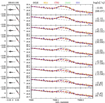
Fig. 7. Nine simulations of OGLE-2016-BLG-1195, similar to Fig. 4, except that in this case the data points are based on the re-reduced data in order to focus on whether the event (once recognized as interesting) would be publishable.
Fig. 7 shows 9 panels with log(q′/q)=−0.05,−0.10, . . .−0.45 , with re-reduced
data from both MOA and KMTA. In each panel, we show both the planetary (2L1S) and binary source (1L2S) models. The number in parentheses to the right of each
log(q′/q) =−0.30 , −0.35 , and −0.40 , these are 17.6, 13.6, and 9.7 respectively. Given that two independent data sets are contributing to these values and that nei-ther shows any sign of systematics, we conclude that the first two would be consid-ered adequate for a reliable detection of a planet, while the third would not.
Next, we address the role of the real time alert. If the event were not recognized in real time at lower mass ratio (as it was in the actual case) then the only
differ-ence in the evaluation of publishability would be the “exclusion” of ≈10 MOA
points during the second half of the anomaly (plus some post-anomaly points),
which would imply slightly lower ∆χ2. In particular, for log(q′/q) =−0.30 and
−0.35 ,∆χ2=13.1 and 10.2, respectively. By the argument just given, these would
render the first as a publishable planet and the second not. Hence, the only
rele-vant question about real-time alerts is whether, at log(q′/q) =−0.35 , the event
would have been alerted based on the online MOA data. Given that the actual event was not recognized by the observers until the deviation was nearly at peak, and so
with roughly twice the deviation as the log(q′/q) =−0.35 case, we regard this as
highly unlikely. Thus, we conclude that the threshold for detection/publication is log(q′/q) =−0.30 .
Finally, we analyze the simulated log(q′/q) =−0.30 as though it were a real
event. We find that there is a unique minimum and that σ(log q) =0.10 . Hence, it
clearly meets our criterion (2).
OGLE-2013-BLG-0341
OGLE-2013-BLG-0341 was originally recognized as having a minor-image
planetary anomaly at HJD′=6393.7 based on real-time OGLE data, four days
after the anomaly, when A.G. cataloged it as a possible high magnification event and therefore carefully examined the light curve as part of his assessment. He pub-licly announced this but also noted that since the lower limit on the magnification,
Amax>10 , was not particularly high, no immediate action was warranted.
How-ever, from this point on, the event was closely monitored with the aim of organizing intensive follow-up observations near peak, if indeed its prospective high-mag char-acter was confirmed. Such intensive observations were in fact initiated ten days after the anomaly and about two days before peak. The peak was characterized primarily by a binary (not planetary) caustic. However, Gould et al. (2014) later showed that the planet’s parameters could be recovered even when the data points in the vicinity of the planetary anomaly (144 points to be precise) were removed from the data.
Nevertheless, because the event eventually did become high-magnification, the light curve would have been singled out for extremely close inspection, regardless of whether a planetary anomaly had previously been noticed or not. If the planet had been noticed at this point, then of course exactly the same follow-up observa-tions would have been initiated. If not, then when the event showed very obvious binary-like behavior (see Fig. 1 of Gould et al. 2014), the event would have been abandoned as “not interesting”. Hence, the signature from the planet in the caustic
exit would have been drastically reduced due to lack of follow-up data4.
In brief, an important (though as we shall see, not only) question of whether the planet would have been recognized comes down to: would Gould et al. (2014) have recognized the planetary signature once they began closely examining this high-mag event, as it approached peak?
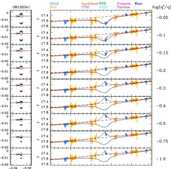
Fig. 8 shows nine panels with log(q′/q) =−0.05,−0.10,−0.15,−0.2,−0.3,
−0.4,−0.5,−0.75,−1 . This event is unique in our sample in that as q declines,
the anomaly becomes less visible and then invisible, but then begins to become
more visible again at log(q′/q) =−0.3 . Then, at log(q′/q) =−0.5 , its visibility
peaks, whereupon it gradually declines. The reason for this behavior is that in the actual event, the source passed along the trough between the two triangular, minor-image caustics, but very close to one of the caustic walls. The source trajectory relative to the mid-line of the trough remains basically the same as q declines, but because the triangular caustics move closer together, the edge of the source moves increasingly over the caustic wall. At first, the excess magnification of the limb increasingly cancels the dip due to the main part of the source passing through the trough. However, when q falls sufficiently, the excess magnification starts to dominate, and there is a bump in place of the trough.
The scatter in the OGLE online data for the six points on the night of the
anomaly is small, σ=0.03 mag. Hence, a mean deviation of just 0.06 mag
would be a five-sigma detection, which we regard as the minimum needed to be both recognizable by eye and to engender sufficient confidence to trigger a massive follow-up campaign, as discussed above. This threshold has already been crossed
at log(q′/q) =−0.15 for the “fading” dip. It is crossed again for the “rising” bump
at log(q′/q) =−0.3 and then is crossed again for the “fading” bump slightly
be-4With respect to the coverage of the caustic, both the OGLE and MOA “survey” data must be
Fig. 8. Nine simulations of OGLE-2013-BLG-0341, similar to Fig. 4. Similar to those simulations, it is based on “online” OGLE and MOA data in order to focus on the problem of real-time recognition of the planetary anomaly.
low log(q′/q) =−0.75 . We conclude that follow-up observations would have been
triggered in the two ranges (log(q′/q)>−0.1) and(−0.3>log(q′/q)>−0.75). Nevertheless, we now argue that only in the former range would a paper claim-ing secure detection of a planet have been written. First, in contrast to a dip in the light curve (which can only be explained by a minor-image anomaly), an iso-lated bump in the light curve can also be explained by a 1L2S solution. The OGLE anomaly data are confined to a narrow range in time, and so have no leverage on the shape of the bump to distinguish between 2L1S and 1L2S.
In principle, the follow-up data (which we argued above would have been trig-gered for the second – “bump” – range of q ) could have confirmed the planetary nature of the anomaly. However, there are two practical issues that severely
under-mine this possibility. First, at our finally adopted value of log(q′/q)≤ −0.1 , we
we return below. More fundamentally, it is very unlikely that the analysis would have been pushed to the point that the test would have been devised of deleting the planetary-anomaly data. The analysis of the event was quite complex and required enormous human and computer resources. It was only in the process of carrying out this analysis that it was discovered that such confirmation was possible. Hence, the motivation to analyze an event to this level in the case that there was a (seem-ingly) unassailable non-planetary interpretation would almost certainly have been lacking. Finally, even supposing that such an analysis were done, the
“confirma-tion” of ∆χ2<50 would almost certainly not have been regarded as sufficient to
claim a secure detection. This is reflected in the fact that Gould et al. (2014) specif-ically argued that the unambiguous planetary anomaly (due to the fact that it was a minor-image dip) served as “confirmation” that the subtle – and by eye, invisible – deviations in the binary caustic could be regarded as a reliable indicator of a planet.
Without such independent knowledge, and at relatively low ∆χ2, this would have
at best led to the reporting of an interesting planetary candidate.
We conclude that the threshold for planet detection is log(q′/q) =−0.10 . We
confirm that this solution is unique and find σ(log q) =0.04 , implying that our
sample criteria are satisfied at this threshold5.
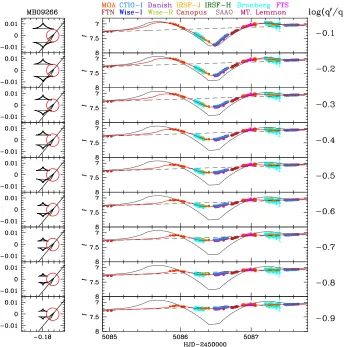
MOA-2009-BLG-266
MOA-2009-BLG-266 (Muraki et al. 2011) was recognized as having a poten-tially planetary anomaly in real time by the MOA collaboration at the end of the New Zealand night from the sharp decline in the previously smoothly rising light curve. This triggered follow up observations at many sites, which further artic-ulated the decline, mapped the trough and then the rise. The basic model of the event was already derived before any of these follow-up data were taken, let alone reduced, so that in the actual case, the alert-generated data were needed for full characterization of the planet, but not for its discovery. However, if the mass-ratio had been lower, it is possible that the planet could not have been characterized well enough to warrant publication in the absence of the follow-up data. Thus, for this event, it is especially important to evaluate both how well the planetary perturba-tion could have been recognized in real time, and how well the planet could have been characterized with, and without, follow-up observations.
We note that five different observatories took data on MOA-2009-BLG-266 prior to the alert, of which four also took data after the alert. Hence, one must assess whether these four would have taken data in the absence of the alert. We find that only one of these (Canopus) took data in a way that indicated sustained
5We note that OGLE-2013-BLG-0341 was part of the Shvartzvald et al. (2016) sample of events
focus on the event as it approached peak: they took four points spread over 1.4 hr on the night before the alert. The others either took one point on occasional nights or had stopped taking data altogether. Thus, it is reasonable to suppose that Canopus would have also taken four points on the next night, even if there had been no alert. However, these data would have overlapped MOA data and so would not have qualitatively altered how well the event could have been characterized in the absence of an alert (and so absence of data in the trough).
Fig. 9. Nine simulations of MOA-2009-BLG-266, similar to Fig. 4. The simulations are based on re-reduced data from all observatories.
Fig. 9 shows nine panels with log(q′/q) =−0.1,−0.2, . . .−0.9 and all data
re-reduced. The first question is whether, with a smaller mass ratio, MOA would have issued an alert (based, of course, on online data). While Fig. 9 shows re-reduced data, it still enables us to understand how the basic form of the MOA light curve
evolves as q declines: over the range log(q′/q)≤ −0.6 , it basically takes the form
anomaly of this form would give rise to an alert provided that the mean excess over the predicted point-lens light curve was 0.1 mag.
Based on the MOA online data from before the night of the anomaly, we find that one can predict the flux (based on a point-lens model) on the night of the
anomaly to 0.085 mag at 3σconfidence. There are ten MOA points on that night,
with scatter 0.024 mag. Hence a standard error of the mean of 0.008 mag. Thus, a
mean offset of 0.1 mag would yield a∆χ2≈12 discrepancy, which would be
suf-ficient indication to issue an alert. This condition is satisfied for log(q′/q) =−0.6 ,
but not lower mass ratios. At higher mass ratios, the mean offset itself satisfies this condition, and in addition there is increasing evidence of a decline (which is what triggered the actual alert).
We fit simulated data for the case log(q′/q) =−0.6 , and find that the solution
is both unique and well localized (σ(log q) =0.02 ). We then repeat this exercise
for log(q′/q) =−0.7 but with only MOA and Canopus data (since, as we argued
above, there would be no alert and hence no follow-up data apart from Canopus). We find that there are several local minima from the broad search of parameter space, and that none of the models derived at these minima appear compelling enough to warrant publication.
We conclude that the threshold for this event is log(q′/q) =−0.6 .
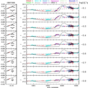
OGLE-2007-BLG-368
The details of the anomaly alert of OGLE-2007-BLG-368 are recounted by Sumi et al. (2010). The first alert was given by the robotic SIGNALMEN anomaly
detector (Dominik et al. 2007) HJD′=4302.314 , being triggered by the nine MOA
points that lie ≈0.2 mag below the point-lens model. This alert prompted
follow-up observations beginning five hours later in Chile by the µ FUN SMARTS 1.3-m telescope and the PLANET Danish 1.5-m, and then from additional telescopes con-tinuing toward the west. From the present perspective, it is important to note that this alert did not reach the MOA observer and so did not influence the cadence of
MOA observations on the night HJD′≈4303 . These were the next observations
after those in Chile. Hence, the next observations that were influenced by the alert (after Chile) were from the PLANET Canopus observations from Tasmania, whose three closely spaced points basically overlap the last MOA point. There were addi-tional follow-up observations, which played an important role in characterizing the
actual event, but as we will show, these play very little role in the current V/Vmax
analysis.
Fig. 10 shows nine panels with log(q′/q) =−0.1,−0.2, . . .−0.9 and all data
re-reduced. Note that for log(q′/q)≤ −0.4 , the point-lens model and the
plane-tary model are nearly identical for the follow-up data taken HJD′>4303.3 . That
is, only the µ FUN Chile, Danish Chile, and Canopus data would have played a
Fig. 10. Nine simulations of OGLE-2007-BLG-368, similar to Fig. 4. This figure is based on re-reduced data from all observatories. It should be compared to the next one (Fig. 11), which is based on “online” OGLE and MOA data.
Fig. 11 shows the same nine panels as Fig. 10 but with only online survey data. Based on this figure, we consider it to be unlikely that there would have been
an alert on this event in time to trigger CTIO observations for log(q′/q)≤ −0.4 .
Moreover, we can say with near certainty (since A.G. made this decision) that CTIO would not have responded to such an alert if it had been given. However, the CTIO response is of secondary importance because the Danish data, which cover the same time interval, would certainly have been taken.
As usual, we first ask at what threshold would the online survey data have led to re-reductions, and then ask whether these reductions would have led to a publishable result given the data that would have been acquired.
The online OGLE data would, by themselves, certainly have triggered
re-reduc-tions at log(q′/q)≥ −0.4 . At log(q′/q) =−0.5 this is less probable, but in this
case the partial corroboration from online MOA data would have almost certainly
Fig. 11. Nine simulations of OGLE-2007-BLG-368, similar to Fig. 4. This figure is based on “online” OGLE and MOA data. It should be compared to the previous one (Fig. 10), which is based on re-reduced data from all observatories.
Recall that at log(q′/q) =−0.3 , we concluded that there would have been an
anomaly alert. We analyze all data and find that the solution is well-localized with
σ(log q) =0.025 . At log(q′/q) =−0.4 , we must consider two cases, i.e., with and
without the alert (and so follow-up data). We find that with the follow-up data,
the minimum is well localized withσ(log q) =0.08 , so satisfying all our criteria.
However, with survey-only (re-reduced) data, we find that there are two minima
separated by ∆χ2<10 and ∆log q>0.3 , which would fail our third criterion.
Since we assessed that there would probably not be an alert at log(q′/q) =−0.4 ,
we conclude that the threshold for detection is log(q′/q) =−0.3 . We recognize
that there is some probability of an alert at log(q′/q) =−0.4 , and therefore
OGLE-2005-BLG-390
[image:30.612.121.467.278.617.2]OGLE-2005-BLG-390 was detected primarily in follow-up data organized by the PLANET collaboration, but in contrast to all previous cases, all of these data were taken in response to an alert of the microlensing event itself, not an anomaly (Beaulieu et al. 2006). The anomalous behavior was noted by the observer at the Danish telescope in Chile, and in principle this could have influenced other obser-vatories farther to the west. PLANET conducted (but did not formally report) an investigation of this question at the time and found that their internal alert did not induce changes in the observing cadence at Canopus (in Tasmania), but did lead to an increased cadence at Perth. However, from the actual record of observations, the observational cadence at Perth did not in fact change from what it had been on previous nights. While in principle it is possible that the internal alert caused a previous decision to reduce the cadence to be exactly revsersed, there is no specific report of such a coincidence. Hence, we believe a more likely explanation is that