Extended Finite Element Modeling: Basic Review and
Programming
Yazid Abdelaziz, K. Bendahane, A. Baraka University of Bechar, Bechar, Algeria
E-mail: [email protected]
Received November 2, 2011; revised June 8, 2011; accepted June 20, 2011
Abstract
In this work, we have exposed a recent method for modeling crack growth without re-meshing. The main advantage of this method is its capability in modeling discontinuities independently, so the mesh is prepared without any considering the existence of discontinuities. The paper covers the formulation and implementa-tion of XFEM, and discusses various aspects of the approach (enrichments funcimplementa-tions, level set representaimplementa-tion, numerical integration…). Numerical experiments show the effectiveness and robustness of the XFEM im-plementation.
Keywords:X-FEM, Programming, Fracture, Cracks, LSM
1. Introduction
The method finite element is widespread in applications of industrial design, and much of various software pack-ages based on techniques of FEM were developed. It proved appropriate for the study of the fracture mechan-ics. However, modelling the propagation of a crack by a finite element mesh proves to be difficult because of the topology alteration of the mesh. Besides, the singularity of the crack end has to be represented exactly by the ap-proximation [1].
Recently a new class has been proposed that simulates the singular nature of discrete models within a geometri-cally continuous mesh of finite elements. The extended finite element method XFEM has emerged from this class of problems, and is based on the concept of parti-tion of unity for enriching the classical finite element approximation to include the effects of singular or dis-continuous fields around a crack [2]. An overview of the early developments of the X-FEM method has been given by Abdelaziz [3,4].
2. Basic Works
The method of X-FEM originators were Belytschko and Black [2]. They introduced a method to develop the fi-nite approximations element so that problems of the crack progression could be solved with remeshing mini-mal. Dolbow et al. [5] and Moes et al. [6] came up with
a more clever technique by adapting an enrichment in-cluding asymptotic at the field and a Heaviside function of H(x).
A significant advance of the extended finite element method was given by its coupling with level set methods (LSM): The LSM is employed to represent both the crack position and that of the crack ends. The X-FEM is employed to calculate the fields of stress and displace-ment that is important to determine the crack growth ratio [7].
The results of the X-FEM method have been so en-couraging that some authors have immediately seized the opportunity to apply this method for solving many kinds of problems where discontinuities and moving bounda-ries are to be modeled.
3. Key Ideas
3.1. X-FEM Approximation
In the X-FEM method, a standard displacement based finite element approximation is enriched by additional functions using the framework of partition of unity ( Fig-ure 1).
4 4
1 1 2 2
1 1 2 1
i i j j
i I j J
l l
k k l k k l
k K l k K l
u u N b N H x
N c F x N c F x
where
Ni is the shape function associated to node i,
I is the set of all nodes of the domain,
J is the set of nodes whose shape function support is cut by a crack,
K is the set of nodes whose shape function support contains the crack front,
ui are the classical degrees of freedom (i.e.
displace-ment) for node i,
bj account for the jump in the displacement field
across the crack at node j. If the crack is aligned with the mesh, bjrepresent the opening of the crack,
H(x) is the Heaviside function,
ckl are the additional degrees of freedom associated
with the crack tip enrichment functions Fl,
Fl is an enrichment which corresponds to the four
as-ymptotic functions in the development expansion of the crack tip displacement field in a linear elastic solid (Figure 2).
3.2. Tip Element
The nodes whose the corresponding shape function sup-port contains the crack tip are enriched by singular func-tions that can model the singular behavior of the dis-placement field at the crack tip.
The crack tip enrichment functions in isotropic elastic-ity Fi(r, ) are obtained from the asymptotic displace-ment fields:
41 sin 2 cos 2 , sin sin 2 cos sin 2 j j r r F r r r (2)
Note that the third singular function F3 is the only
en-richment function which is discontinuous across the crack. Thus, the discontinuity of the displacement field at
π
in the singular enrichment zone is only modeled by F3 on the element containing the crack tip.
3.3. Split Element
The nodes whose the corresponding shape function sup-port is totally cut by the crack, are enriched by an Heaviside function (Figure 3).
The function of Heaviside jump is a discontinuous function through the surface of slit and constant on both slit sides: +1 on a side and –1 on the other.
e i a e i b i u Crack Crack tip i
u : Classical element. e
i
a : Split element.
e i
[image:2.595.310.538.77.487.2]b : Tip element.
[image:2.595.92.224.432.545.2]Figure 1. X-FEM enrichment strategy.
Figure 2. 2D view of near tip asymptotic functions.
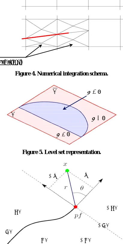
[image:2.595.307.539.520.706.2]3.4. Numerical Integration
For the slit cut elements that are enriched with the jump function H(x), Moes [6] altered the routines quadrature element for the weak form assembly. Because the slit can be randomly directed in an element, the standard squar-ing of Gauss may not properly integrate the field of dis-continuity. This process is generally carried out by means of dividing them into standard sub-triangles (Fig-ure 4). Consequently whenever the slit propagates, a
new sub-triangles set and a new set of gauss points are used.
4. Method of the Level Set
The description of discontinuities in the context of the extended finite element method is often realized by the level-set method. The Method of level set is a numerical design of Osher [8] for interfaces movement modeling. The method is believed to represent an interface by the zero of a function, called the function of the level set, and the Hamilton-Jacobi’s equations modernized the function of the level set so as to know the interface speed in the normal direction to this interface (Figure 5).
A crack is described by two level sets (Figure 6): a normal level set, (x), which the signed distance to
the crack surface,
a tangent level set (x), which is the signed distance to the plane including the crack front and perpendicular to the crack surface.
In a given element, min and max, respectively, be the
minimum and maximum nodal values of on the nodes of that element. Similarly, let min and max, respectively
be the minimum and maximum nodal values of on the nodes of an element:
If < 0 and minmax 0, then the crack cuts through
the element and the nodes of the element are to be en-riched with H(x).
If in that element minmax 0 and minmax 0, then
the tip lies within that element, and its nodes are to be enriched Fi(r, ).
5. Programming Procedure
One can apply the method of finite extended element within one finite element code with relatively slight al-terations: variable degrees numbers of freedom per node; interaction of mesh geometry (a manner to detect ele- ments intersecting with discontinuity geometry); matri-ces of enriched rigidity; numerical integration. Sukumar and Prévost [9] described the X-FEM execution to model discontinuities of cracks within Dynaflow [10], as a package of standard finite element. Huang et a1. [11]
[image:3.595.319.531.64.229.2]Sub-triangle Crack
Figure 4. Numerical integration schema.
0
0
0
Figure 5. Level set representation.
φ < 0 φ > 0
φ = 0
ψ < 0
ψ > 0
ψ = 0 φ(x)
ψ(x)
Figure 6. Coupling XFEM/LSM.
concentrated on the X-FEM application to problems of cracks in isotropic and bi-material media. Nisto et al.’s suggestion [12] of a numerical establishment in an ex-plicit code was to treat the propagation of active cracks. The explicit dynamic FEM code (DynELA) [13] devel-oped in the LGP with an object-directed framework to support the X-FEM application as a new module called DynaCrack. Bordas extended finite element library [14], the structure program, was conceived to fit all natural modularity, extensibility and robustness requirements. (C++) and of a commercial package of solid modeling/ finite element.
[image:3.595.321.526.120.525.2]element code with relatively small modifications: vari-able number of degrees of freedom per node; mesh ge-ometry interaction; enriched stiffness matrices; numeri-cal integration [9].
1) Input data: defining various object entities (crack, holes, inclusions, interfaces…), enrichment types and crack growth law.
2) Nodal degrees of freedom: a part from the classical degrees of freedom, additional unknown enriched de-grees of freedom is introduced via the displacement ap-proximation.
3) Mesh-geometry interactions: This sub-category de-tects the selection of the enriched nodes, then touches upon the computation of enrichment functions, and de-tects the partitioning of the finite elements that are inter-sected by the crack.
4) Assembly procedure: The stiffness matrix and force vector assembly are done on an element level, which is similar to classical finite element implementation. The distinction herein is that the dimensions of the element stiffness matrix can differ from element (unenriched) to element enriched).
5) Post-processing: This sub-category addresses the main objectives of a fracture analysis by determining the interaction integral, and controlling the crack growth criteria.
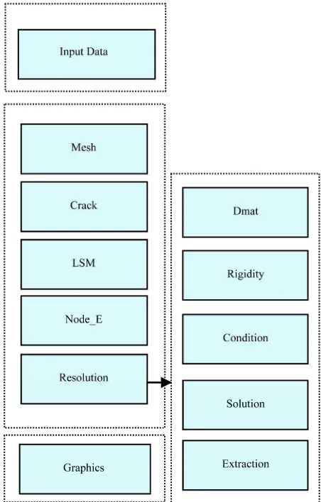
The task of incorporating the X-FEM capabilities within a general-purpose finite element program can be broken down into the following schema (Figures 7 and 8, Table 1):
6. Numerical Experimentation
The Figures 9, 10, 11 and 12 show tow examples of
crack growth modeling without re-meshing obtained by X-FEM code.
7. Conclusions
[image:4.595.310.536.79.433.2]The extended finite element method (X-FEM) uses the partition of unity to remove the need to mesh physical surfaces or to remesh them as they evolve. It allows to model cracks, material inclusions and holes on non con-forming meshes. The methodology of X-FEM that dif-fers from that of the traditional method of finite element is of very particular concern since it does not force dis-continuities to go with the borders. It solves the techno-logical problems in the various complex fields accurately; the thing that can hardly be achieved impossible when using the traditional method of finite element alone. In this work, we present the basic concepts and the implan-tation of the X-FEM. The work discusses general algo-rithms for implementing an efficient X-FEM. A numerical
[image:4.595.309.539.463.705.2]Figure 7. Structural scheme of the X-FEM code.
Table 1. List of X-FEM functions.
List Description
Input Input data
Mesh Mesh generation
Crack Determination of the tip segment
LSM Level set
Node_E Extraction of the enriched node
Resolution Construction and solving of linear equations
Graphics Plotting
Dmat Constrictive matrix
Rigidity Compute stiffness matrix
Condition Boundary condition
Solution Solution of equations
Extraction Stress intensity factors computation
Int_H Partition of the crack split element
Int_F Partition of the crack tip element
Gauss Gauss quadrature
Bmat Stiffness Matrix computation
Delaunay Delaunay triangulation
Function Shape function
Func_H Crack split element enrichment
[image:5.595.59.291.88.706.2]Func_P Crack tip element enrichment
[image:5.595.308.541.297.477.2]Figure 9. Crack growth modeling by X-FEM (SEN speci-men)
[image:5.595.309.541.515.696.2]Figure 10. Crack growth modeling by X-FEM (CN speci-men).
Figure 11. Stress distribution for different crack lengths (SEN specimen).
experiment is provided to demonstrate the effectiveness and robustness of the X-FEM implementation.
8. References
[1] P. Tong and T. Pian, “On the Convergence of the Finite Element Method for Problems with Singularity,” Interna-tional Journal of Solids and Structures, Vol. 9, No. 3,
1973, pp. 313-321.
[2] T. Belytschko and T. Black, “Elastic Crack Growth in Finite Elements with Minimal Remeshing,” International Journal for Numerical Methods in Engineering, Vol. 45, No. 5, 1999, pp. 601-620.
[3] Y. Abdelaziz and A. Hamouine, “A Survey of the Ex-tended Finite Element,” Computers and Structures, Vol. 86, No. 11-12, 2008, pp. 1141-1151.
[4] Y. Abdelaziz, A. Nabbou and A.Hamouine, “A State-of-the-Art Review of the X-FEM for Computational Fracture Mechanics,” Applied Mathematical Modelling, Vol. 33, No. 12, 2009, pp. 4269-4282.
[5] J. Dolbow, “An Extended Finite Element Method with Discontinuous Enrichment for Applied Mechanics,” PhD Thesis, Northwestern University, Chicago, 1999. [6] N. Moes, J. Dolbow and T. Belytschko, “A Finite
Ele-ment Method for Crack Growth without Remeshing,” In-ternational Journal for Numerical Methods in Engineer-ing, Vol. 46, No. 1, 1999, pp. 131-150.
[7] M. Stolarska, D. D. Chopp, N. Moes and T. Belyschko, “Modelling Crack Growth by Level Sets in the Extended Finite Element Method,” International Journal for
Nu-merical Methods in Engineering, Vol. 51, No. 8, 2001, pp.
943-960.
[8] S. Osher and J. Sethian, “Fronts Propagating with Curva-ture Dependent Speed: Algorithms Based on Hamil-ton-Jacobi Formulations,” Journal of Computational Physics, Vol. 79, No. 1, 1988, pp. 12-49.
[9] N. Sukumar and J. H. Prevost, “Modeling Quasi-Static Crack Growth with the Extended Finite Element Method Part I: Computer Implementation,” International Journal of Solids and Structures, Vol. 40, No. 26, 2003, pp.
[10] J. Prevost, “Dynaflow,” Princeton University, Princeton, 1983.
[11] R. Huang, N. Sukumar and J. Prevost, “Modeling Quasi-Static Crack Growth with the Extended Finite Element Method Part II: Numerical Applications,” Inter-national Journal of Solids and Structures, Vol. 40, 2003,
pp. 7539-7352
[12] I. Nistro, O. Pantale and S. Caperaa, “On the Modeling of the Dynamic Crack Propagation by Extended Finite Ele-ment Method: Numerical Implantation in DYNELA Code,” 8th International Conference on Computational Plasticity, Barcelona, 5-8 September 2005.
[13] O. Pantale, S. Caperaa and R. Rakotomalala, “Develop-ment of an Object Oriented Finite Ele“Develop-ment Program: Ap-plication to Metal Forming and Impact Simulation,” J-CAM, Vol. 186, No. 1-2, 2004, pp. 341-351.