An adaptive hybrid force/motion control design for robot manipulators interacting in constrained motion with unknown non rigid environments

An Adaptive Hybrid Force/Motion Control Design

for Robot Manipulators Interacting in Constrained

Motion with Unknown Non-Rigid Environments

Aghil Jafari and Jee-Hwan Ryu

School of Mechanical Engineering Korea University of Technology and Education

Cheonan, Rep. of Korea, 303-708 Email: Jafari_ [email protected]@kut.ac.kr

Ali Talebi

Department of Electrical Engineering Amirkabir University of technology

Tehran, Iran Email: [email protected]

Abstract-In the present paper, the objective of hybrid control is specified and an adaptive hybrid force/motion control approach is proposed. Based on the concept of hybrid control, the task space is decomposed into position and force controlled subspaces. An adaptive scheme is presented which makes the controller robust when the robot is in interaction with an unknown non­ rigid environment. By using the classical Lyapunov method, it is demonstrated that the proposed control law ensures the tracking of the unconstrained components of the desired end-effector trajectories, with regulation of the desired contact force along the constrained direction. Simulation results verify the effectiveness of our prosperous adaptive hybrid control in robot-environment interaction.

Keywords-Hybrid Control, Adaptive Control, Robot­ Environment Interaction, Robust Control.

I. INTRODUCTION

During the last two decade, the control of robot envi­ ronment interaction (also known as compliant motion) has emerged as one of the most attractive and fruitful research area in robotic. In all of these applications the position and in­ teraction force of end-effector manipulator must be controlled simultaneously. The initial investigations in the field were motivated by practical needs for automating complex tasks mainly performed by human, such as assembly, deburring, etc. The control of physical robot interaction is still a challenging research issue, recently addressing the emerging fields of human-robot interaction systems, human augmentations and enhancements, haptic rendering, rehabilitation robotics, etc [1].

In the hybrid force/position control strategy, either a posi­ tion or a force is controlled along each task space direction, through the use of proper selection matrices [2, 3]. Considering parametric uncertain robot manipulators, several robust control strategies [4, 5, 6] provide asymptotic motion tracking and an ultimate bounded force error. In addition, Kiguchi [7] and Song

Mehdi Rezaei and Reza Monfaredi Department of Mechanical Engineering

Amirkabir University of technology Tehran, Iran

Email: [email protected][email protected]

Saeed Shiry Ghidary

Department of Computer Engineering Amirkabir University of technology

Tehran, Iran Email: [email protected]

[8] accordingly utilize the fuzzy neural networks and variable structure control to compensate the environmental friction.

To deal with uncertainty in system dynamics, an adaptive controller was proposed in [9] where measurement of joint accelerations was used. This requirement was relaxed later in [10], but the adaptation law was not sensitive to force changing since it did not have force error in its structure. We especially note here that Yoshikawa and Sudou [11] developed a dynamic hybrid position/force control scheme to deal with an unknown constraint. The difficulty for considering an uncertain constraint is that the motion and force control designs are no longer decoupled. In this case, the above developed adaptation law cannot be applied. This led to complex strategies in [12, 13]. In [14] a systematic adaptive control strategy based on the concept of virtual decomposition was introduced to handle a variety of control objectives. An adaptive synchronized control approach was presented in [15] to address the coordination problem when the robots are in contact with a frictionless surface with unknown geometry.

Most robust approaches, [16, 6], etc., were proposed by utilizing discontinuous control laws, which arise some draw­ backs. To the best of our knowledge, not many works provide disturbance attenuation for both motion and force tracking based on continuous control laws. For example, Chang and Chen [17] applied the adaptive fuzzy technique to achieve ro­ bust motion tracking performance for constrained mechanism. Although vast researches of the Hoo control technique [18, 19, 20, 21] have be conducted, all the methods did not deal with a robust performance criterion involving non-dynamical variables like force errors. Consequently, the disturbance at­ tenuation problem for force error is not trivial.

The main advantage of the proposed controller is requiring no measurement of force derivative or acceleration signal in the adaptation law design comparing to the latest research in the field and the controller is simple in the structure yet. The dynamics and related properties for constrained robot manipulators are addressed in Section (II). In Section (III), an adaptive motion/force tracking problem is formulated, where an adaptive controller is developed. Section (IV) shows a complete stability proof, based on the Lyapunov direct method. Section (V) shows the simulation results for controlling a planar revolute robot in constrained motion. Finally, some conclusions are made in Section (VI).

II. DYNAMICS FORMULATION

The dynamics of a rigid robot manipulator are described in the task space by the equation [9]:

Mx(x)x + Cx(x, x)x + dx(x, x) + gx(x) =

u

-f

(1)

Where

x

is the (m xl) vector of task variables (usually

the end-effector location),

Mx

is the (m x m) symmetric

inertia matrix,

Cxx

is the (m xl) vector of Corio lis and

centrifugal generalized forces,

dx (x, x)

is the (m xl) vector

of forces generated by joint friction,

gx

is the (m xl) vector

of gravitational generalized forces, u is the (m xl) vector

of driving generalized forces, and

f

is the (m xl) vector

of contact generalized forces exerted by the manipulator on the environment; all task space quantities are expressed in a common reference frame.

The

(n

x 1) vector T of joint-actuating generalized forces can be computed as

(2)

where q is the

(n

xl) vector of joint variables and

J

is the

(m x

n)

manipulator Jacobian matrix.

Two notable properties of the dynamic model (1) can be established [2]:

• _{There exists a choice of the matrix}

Mx

_{such that the} matrix

S(x,x) = Mx(x) -2Cx(x,x)

(3)

is skew-symmetric.

• _{The dynamic model (1) is linear in terms of a suitable}

set of dynamic parameters, i.e.,

Mx(x)x+Cx(x, x)x+dx(x, x)+gx(x) = Yx(x, x, x)e

(4) where

Yx (x, x, x)

is an (m x p) regressor matrix and

e

is a (p xl) vector of manipulator and load dynamic parameters

III. CONTROL DESIGN

Consider the following control law

u

= Mx(x)r + ex(x, x)r + dx(x, x) + 9x(X) - kD(X -r) + f

(5) where

Mx, ex, dx

and

9x

are the estimates of

Mx, ex, dx

and

9x,

respectively,

f

is the measured contact force,

r

is a (m x 1) reference vector, and

Kd

is a positive definite matrix.

Using the second property of the dynamic model (4), the control law (5) can be written as

u

= Yx(x, x, r, r)e - kD(X -r) + f

(6)

Notice that the matrix

ex

in (5) must satisfy a property analogous to the skew-symmetry of the matrix in (3). Com­ bining (1) with (6) gives

Mx(x)e+Cx(x,x)e+dx(x,x,e)+kDe = Yx(x,x,r,r)e

(7)

where

dx = dx -dx, e = e -e,

and

r=x -e

r=x -e

(8)

(9)

On the assumption that

dx

contains only viscous and static friction, it can be shown that [9]:

T-e dx(x, x, T-e)

� 0 (10)

To obtain a force/position controller, the error vector

e

should be properly related to the force and position errors. The parallel control strategy suggests relating the error vector in (8) to both position and force error, without using any selection mechanism [9]. Along the constrained task directions, the conflict between the position and force actions must be managed by imposing dominance of the force action over the position one.

Let

Xd, Xd

and

Xd

denote the time-varying desired end­ effector position, velocity and acceleration, respectively. Let also

fd

denote the constant desired force vector. The error between the actual and desired end-effector positions is indi­ cated by

�x = x -Xd,

and

�f = f -fd

indicates the error between the actual and desired contact forces. To implement hybrid position/force control, a diagonal Boolean matrix

S,

called the compliance selection matrix [9], has been introduced and in accordance with the specified artificial constraints the i-th diagonal element of this matrix has the value 1 if the i-th DOF with respect to the task-frame is to be force-controlled, and the value 0, if it is position-controlled.

An effective choice for the error vector in (8) is t

e =

(I

-S)(�X+AI�X)+S(�j+AI�f +A2

J

�f d t)

(11)

o

where

AI, A2 >

O.

It is worth noticing that

�x

and

�f

are not independent, since they are constrained by the contact with the environment. Without loss of generality, the case of m

= n =

3 is taken, i.e.,

only translational motion and force components are considered. The environment is thought of as a frictionless elastic plane. Hence, the model of the contact force takes the simple form

f = K(x -xo)

(12)

where

x

is the position of the contact point,

Xo

is a point of the plane at rest, and

K

is the (3 x 3) constant symmetric stiffness matrix that can be expressed as

where k is the stiffness coefficient and we assume that it is positive and unknown, but it has a known upper band

(kmax). n is the unit vector orthogonal to the contact plane. These are assumed to be constant. In addition, we assume that the environment has one dimension; consequently, the selection matrix can be written as

(14)

As a further assumption, it is supposed that the contact between the manipulator and the environment is not lost.

In view of the above consideration and of (12) and (13), the following equilibrium trajectory is obtained:

T Tl

Xe = (I - nn )Xd + nn (I/d + xo) (15)

fe = knnT(Xe -xo) = fd (16)

IV. STABILITY

In order to study the stability of the system (7), (11), (12), and (13) around the equilibrium trajectory (15), (16) with a proper parameter adaptation law, Su is defined as

(17)

Then, from above equation

Su = (I - nnT)fix + nnT fij (18)

In view of (11), Equation (18) can be written in the form

(19)

where

(20)

Differentiating (20) with respect to time and taking into account (12), (13), (16), and (17) yields

. _{T T}

h = n fif = kn Su

At this point, consider the (7 xl) state vector

(21)

(22)

The system described by (7), (19), and (21) can be written in the standard compact form:

(23)

where 0 denotes the (3 x 3) null matrix and

0

the (3 x 1) null

vector.

Notice that an equivalent representation of the system (7),

(19), and (21) can be obtained in terms of the (7 x 1) state

vector

w =

( s�

(24)

through a non-singular state space transformation w = T z

where

T=

(

b

OT

The following result can be stated:

Theorem. Consider the parameter adaptation law

eA _{= -}r-lyT( ' _{x x,x,r,r e} . )

(25)

(26)

where r is a (p x p) symmetric positive definite matrix. There exists a choice of feedback gains Al and

A2

that makes the origin of the state space for the augmented system (23) and

(26) stable. Moreover if Xd, Xd and Xd are bounded, then z -7 o as

t

-7 00.

Proof. Consider the Lyapunov function candidate

Computing the time derivative of V along the trajectories of system (23) and (26) gives

�

)

Tz - eT dx

A2

2

(28)

in which the skew-symmetry of the matrix NIx - 2Cx has been conveniently exploited.

Since the matrix T in (25) is non-singular, and in view of

(10), from (28) it follows that 11 is negative semi-definite if (29)

This choice makes V in (27) positive definite. Therefore (27) is a Lyapunov function and the system (23) and (26) is stable. Moreover, z and e are bounded and e, s E

L�,

h E

L2.

Equations (19) and (21) imply respectively that Su and

h are bounded. It is easy to show that e is also bounded if

fd, Xd, Xd and Xd are bounded. Using Barbalats lemma (Slotine & Li, 1991), it follows that e, sand h are uniformly continuous and z -7

0

as

t

-7 00.

By virtue of the state-space transformation given by (25), the result z -7

0

as

t

-7 00 is equivalent to w -7

0

as

t

-7 00.

Then from (17) and (19) it follows that x -7 Xe and x -7 Xd

as

t

-7 00; from (21) f -7 fd as

t

-7 00.

If the dynamic parameters of the manipulator are known, i.e., iJ = e, a stronger result can be stated.

V. SIMULATION RES ULT

for M ATL AB developed by Corke [22], which includes the kinematic model of the robot.

We consider a typical robot task in which the robot end­ effector realizes the desired motion

Xd(t)

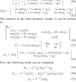
along the x-axis and the required contact force Fd in the y-direction. The environment model defined in the direction perpendicular to the sliding surface (the y-direction in Fig. 1 & 2) is assumed to be in the form of linear elastic. Adopting that

q = [ ql q2 ] T,

neglecting the joints friction, and using the notation given in Fig. 1, the system's forward kinematics and its Jacobian are

[

X

]

_

[

h COS(ql)

+ l2 COS(q1 +

q2)

]

(30)

Y

-

h sin(ql)

+

l2 sin(ql

+

q2)

J(

q -

) - [

-(h sin(ql)

h cos(qI)

₊ +

l2 COS(ql

l2 sin(q1

₊ +

q2)

q2)) -l2 sin(q1

l2 COS(ql

₊ +

q2)

q2)

]

(31) The matrices in the robot dynamics model (1) can be written as:

m2l2(l2

+

2h cos q2)

m2l§

1

(32)

[

-2q2 -q2

Cq = m2hl2 sin(q2)

0

q2

(33)

Gq =

9.81

[

(ml

+

m2)ll COS q1

m2l2 COS(ql

+

m2l2 COS(q1

₊

q2)

+

q2)

l

34) Now, the following result can be computed:

Mx = JT(q)MqJ-l(q)

(35)

Cx = J-T(q)( Cq -MqJ-1(q)j(q))J(q)

(36)

gx=J-T(q)gq

(37)

The model of active force acting upon the tip of the robots end-effector is represented by the following relation:

-Fy

= ky

(38)

where

k

is the environment stiffness parameter. For a relatively non-rigid environment we assume the following hypothetical values of its parameter;

k =

1700

[Njm] .

The robot links are

h = l2 =

1

[m]

, and their masses

ml =

1.3

[kg]

and m2 = 0.9

[kg] .

Let the unknown parameters

T

vector to be e

= [ m1 m2 ] .

To perform the adaptive hybrid controller, The initial states are set as

q1(0) =

0.657,

q2(0) =

0.913 and

q1(0) = Q2(0) =

O. According to the nominal constraint, the desired motion trajectory

X1d =

1 + 0.1

sin(t) [m]

while the desired normal force is

hd =

1

N.

The control gains are chosen as

Al =

40,

A2 =

0.1 and r

=

70 I where I is the

(2

x

2)

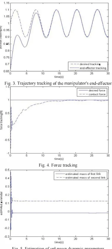
identity matrix.

The simulation result for the motion tracking is shown in Fig. 3. The desired force and constraint force is shown in Fig. 4. These Figs demonstrate the ability of the proposed hybrid controller. The proposed control system with respect to position and contact force ensures the stable desired motion

Xld

of the end-effector on the surface and the desired con­ tact force

hd

along the surface normal vector. Besides, the

Ylm]

xlm]

Fig. 1. Model of a 2-DOF planar manipulator

"

"

"

DO

"

..

Fig. 2. Model of a 2-DOF planar manipulator in Robotic Toolbox of MATLAB

control law ensures both the stability of the desired quality of dynamic behavior in all directions of motion. Fig. 5 shows the adaptation performance of the estimated parameters with the update gains r

=

70 I. It is worth noting that the parameters do not converge to the real values. Instead, it is synthesized so that the tracking errors of the system converge to zero and the estimation error is guaranteed to be bounded. This explains the validity of negative estimated mass of the second link Fig. 5.

VI. CONCLUS ION

An adaptive compliant control scheme for robot manipu­ lators in contact with an elastic surface has been analyzed in this work. The stability of the controller is proved by means of the Lyapunov direct method. A simple condition involving the feedback gains and the surface stiffness guarantees the stability of the controlled system in the sense of Lyapunov. Simulation results on a planar robot manipulator have demonstrated the effectiveness of the control system.

ACKNOWLEDGMENT

[image:4.612.325.567.52.195.2] [image:4.612.49.302.185.459.2] [image:4.612.334.549.232.369.2]

E

115r---�--�--�--�--�----'

1.1 .r\

I \ 1.05 _I I \

\ \ g; 0.95

\

\ -'"

� 0.9

10.85

0.7 ---desired tracking

--end-effector tracking o.65o!--_{----c:------01=-o ----;,':-5 -'===::2'.C'0 ="'=��25���3·0}

lime(s)

Fig. _3. Trajectory tracking of the manipulator's end-effector 1.,

I--'-�--'---�--=--�---'-r======il

1

_-

_{desired force}

---contact force

-0.5

"O�---C:---O'=-O ----;,':-5----:2':-0 ----:2':-5 ----='3·0

time(s)

Fig. _4. Force tracking

O. 5.-�--�-r=============;]

1

_-

estimated mass offirst link

-- -estimated mass of secend link

0.4

0.3

E 0.2

::! _1�

______________________________ _

i 0.1 g

�

-0.1

-0.2

.030';---,:---;,':-0 ----;,':-5 ----:2':-0 ----:2':-5 ----:'3-0 lime(s)

Fig. _5. Estimation of unknown dynamic parameters

REFERENCES

[1] M.Vukobratovic, D.Surdilovic, Dynamics and robust control of robot envirorunent interaction, Singapore, World Scientific, ch. 1&2,2009.

[2] T. Yoshikawa, Dynamic hybrid position/force control of robot

manipulators: Description of hand constraints and calculation

of joint driving force, IEEE 1. of Robotics and Automation,

ch.3, pp. 386-392, 1987.

[3] H. Seraji, Adaptive force and position control of manipulators,

1. of Robotic Systems, VoL 3, pp. 551- 578, 1987.

[4] M. C. Hwang, X. Hu, A robust position/force linearing controller of manipulators via nonlinear Hoo control and neural networks, IEEE Transactions on System, Man, Cybernetics­ Part B, VoL 30, pp. 310-321, 2000.

[5] C. M. Kwan, Robust adaptive force/motion control of

constrained robots, IEEE Proceedings Control Theory and

Application, VoL 143, pp. 103-109, 1996.

[6] R. Y. Zhen, A. A. Goldenberg, Variable structure hybrid control of manipUlators in unconstrained and constrained motion, ASME Journal of Dynamic of System, Measurement and

Control, VoL 118, pp. 327332, 1996.

[7] K. Kiguchi,T. Fukuda, Fuzzy-neuro position/force control of robot manipulators two stage adaptation approach, Proceedings of the IEEE international conference on intelligent robots and

systems , Measurement and Control, pp. 1226-1233, 1999 ..

[8] G. Song, L. Cai, Robust position/force control of robot manipulators during constrained task, iEEE Proceedings on Control Theory and Applications, VoL 145, pp. 427433,1998. [9] B. Siciliano, L. Villani, Adaptive compliant control of robot

manipulators, Control Eng. Practice, VoL 4, No. 5, pp. 705-712, 1996.

[10] C. Chiu, K. Llian, T. Wu, Robust adaptive motion/force tracking control design for uncertain constrained robot manipulator,int. 1. ELSEVIER, Automatica, VoL 40, pp. 2111-2119,2004 .

[Il] T. Yoshikawa, A. Sudou, Dynamic hybrid position/force control of robot manipulators on-line estimation of unknown

constraint, IEEE Transactions on Robotics and Automation,

VoL 9, pp.220226, 1993.

[12] S. Hu, H. Krishnan, NN controller of the constrained robot

under unknown constraint, IEEE 26th annual conference, VoL

9,pp. 2123-2128,2000.

[13] P. R. Pagilla, B. Yu, A stable transition controller for constrained robots, IEEE Transactions on Mechatronics, VoL 6, pp. 6574, 2001.

[14] D. Sun, J.K. Mills, Adaptive synchronized control for coordination of multi-robot assembly tasks, IEEE Transactions

on Robotics and Automation, VoL 18, pp. 498509, 2002.

[15] M. Namvar, F. Aghili, Adaptive Force-motion Control of Coordinated Robots Interacting with Geometrically Unknown Environments, International, IEEE Conference on Robotics & Automation, New Orlan, LA. 2004.

[16] G. Song, L. Cai, Robust position/force control of robot

manipulators during constrained task, IEEE Proceedings on

Control Theory and Applications, VoL 145, pp. 427433,1998. [17] Y. C. Chang, B. S. Chen, Robust tracking designs for both

holonomic and nonholonomic constrained mechanical systems: adaptive fuzzy approach, IEEE Transactions on Fuzzy Systems,

VoL 8, pp. 4666, 2000.

[18] B. S. Chen, T. S. Lee, J. H. Feng, A nonlinear control design in robotic systems under parameter perturbation and external disturbance, International Journal of Control, VoL 59, pp. 439-461,1994.

[19] B. S. Chen, Y. C. Chang, T. C. Lee , Adaptive control in robotic systems with Hoo tracking performance, Automatica, VoL 33, pp. 227234,1997.

[20] G. W. Lee, F. T. Cheng , Robust control of manipulators using the computed torque plus H compensation method, iEEE

Proceedings Control Theory and Applications, VoL 143, pp.

6472,1996.

[21] P. Tomei, Robust adaptive friction compensation for tracking control of robot manipulators, IEEE Transactions on Automatic Control, VoL 45, pp. 21642169, 2000.

[image:5.612.109.297.50.467.2]