SNAP: A Multi Stage XML Pipeline for Aspect Based Sentiment Analysis

SNAP: A Multi-Stage XML-Pipeline for Aspect Based Sentiment Analysis

Clemens Schulze Wettendorf and Robin Jegan and Allan K¨orner and Julia Zerche

andNataliia Plotnikova and Julian Moreth and Tamara Schertl and Verena Obermeyer

andSusanne Streil and Tamara Willacker and Stefan Evert

Friedrich-Alexander-Universit¨at Erlangen-N¨urnberg Department Germanistik und Komparatistik

Professur f¨ur Korpuslinguistik Bismarckstr. 6, 91054 Erlangen, Germany

{clemens.schulze.wettendorf, robin.jegan, allan.koerner, julia.zerche, nataliia.plotnikova, julian.moreth, tamara.schertl, verena.obermeyer,

susanne.streil, tamara.willacker, stefan.evert}@fau.de

Abstract

This paper describes the SNAP system, which participated in Task 4 of SemEval-2014: Aspect Based Sentiment Analysis. We use an XML-based pipeline that com-bines several independent components to perform each subtask. Key resources used by the system are Bing Liu’s senti-ment lexicon, Stanford CoreNLP, RFTag-ger, several machine learning algorithms and WordNet. SNAP achieved satisfactory results in the evaluation, placing in the top half of the field for most subtasks.

1 Introduction

This paper describes the approach of the SemaN-tic Analyis Project (SNAP) to Task 4 of SemEval-2014: Aspect Based Sentiment Analysis (Pontiki et al., 2014). SNAP is a team of undergraduate students at the Corpus Linguistics Group, FAU Erlangen-N¨urnberg, who carried out this work as part of a seminar in computational linguistics.

Task 4 was divided into the four subtasks As-pect term extraction(1),Aspect term polarity(2), Aspect category detection(3) andAspect category polarity(4), which were evaluated in two phases (A: subtasks 1/3; B: subtasks 2/4). Subtasks 1 and 3 were carried out on two different datasets, one of laptop reviews and one of restaurant reviews. Subtasks 2 and 4 only made use of the latter. This work is licensed under a Creative Commons Attribution 4.0 International Licence. Page numbers and proceedings footer are added by the organisers. Licence details: http: //creativecommons.org/licenses/by/4.0/

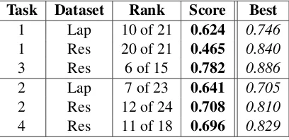
Task Dataset Rank Score Best

1 Lap 10 of 21 0.624 0.746 1 Res 20 of 21 0.465 0.840 3 Res 6 of 15 0.782 0.886 2 Lap 7 of 23 0.641 0.705 2 Res 12 of 24 0.708 0.810 4 Res 11 of 18 0.696 0.829

Table 1: Ranking among constrained systems.

The developed system consists of one module per subtask, in addition to a general infrastruc-ture and preprocessing module, All modules ac-cept training and test data in the XML format spec-fied by the task organizers. The modules can be combined into a pipeline, where each step adds new annotation corresponding to one of the four subtasks.

Table 1 shows our ranking among all con-strained systems (counting only the best run from each team), the score achieved by SNAP (accu-racy or F-score, depending on subtask), and the score achieved by the best system in the respec-tive subtask. Because of a preprocessing mistake that was only discovered after phase A of the eval-uation had ended, results for subtasks 1 and 3 are significantly lower than the results achieved dur-ing development of the system.

2 Sentiment lexicon

Early on in the project it was decided that a com-prehensive, high-quality sentiment lexicon would play a crucial role in building a successful sys-tem. After a review of several existing lexica, Bing

Liu’s sentiment word list (Hu and Liu, 2004) was taken as a foundation and expanded with extensive manual additions.

The first step was an exhaustive manual web-search to find additional candidates for the lexicon. The candidates were converted to a common for-mat, and redundant entries were discareded. The next step consisted of further expansion with the help of online thesauri, from which large num-ber of synonyms and antonyms for existing entries were obtained. Since the coverage of the lexicon was still found to be insufficient, it was further complemented with entries from two other exist-ing sentiment lexica, AFINN (Nielsen, 2011) and MPQA (Wilson et al., 2005).

Finally the augmented lexicon was compared with the original word lists from AFINN, MPQA and Bing Liu in order to measure the reliabilty of the entries. The reliability score of each entry is the number of sources in which it is found.

3 Infrastructure and preprocessing

Within the scope of Task 4 – but not one of the official subtasks – the goal of the infrastructure module was (i) to support the other modules with a set of project-specific tools and (ii) to provide a common API to the training and test data aug-mented with several layers of linguistic annota-tion. In order to roll out the required data as quick as possible, the Stanford CoreNLP suite1

was used as an off-the-shelf tool. The XML files provided by the task organizers were parsed with the xml.etree.ElementTree API, which is part of the standard library of Python 2.7.

Since the module for subtask 1 was pursuing an IOB-tagging approach for aspect term identifica-tion, the part-of-speech tags provided by CoreNLP had to be extended. During the process of merging the original XML files with the CoreNLP annota-tions, IOB tags were generated indicating whether each token is part of an aspect term or not. See Section 4 for further information.

For determining the polarity of an aspect term, the subtask 2 module made use of syntactic depen-dencies between words (see Section 5 for details). For this purpose, the dependency trees produced by CoreNLP were converted into a more accessi-ble format with the help of the Python software packageNetworkX.2_.

1_{http://nlp.stanford.edu/software/corenlp.shtml} 2_{http://networkx.github.io/}

4 Aspect term extraction

The approach chosen by the aspect term extrac-tion module (subtask 1) was to treat aspect term extraction as a tagging task. We used a standard IOB tagset indicating whether each token is at the beginning of an aspect term (ATB), inside an as-pect term (ATI), or not part of an aspect term at all (ATX).

First experiments were carried out with uni-gram, bigram and trigram taggers implemented in NLTK (Bird et al., 2009), which were trained on IOB tags derived from the annotations in the Task 4 gold standard (comprising both trial and training data). We also tested higher-order n-gram taggers and the NLTK implementation of the Brill tagger (Brill, 1992).

For a more sophisticated approach we used RF-Tagger (Schmid and Laws, 2008), which extends the standard HMM tagging model with complex hidden states that consist of features correspond-ing to different pieces of information. RFTagger was developed for morphological tagging, where complex tags such as N.Reg.Nom.Sg.Neut are decomposed into the main syntactic category (N) and additional morpho-syntactic features rep-resenting case (Nom), number (Sg), etc.

In our case, the tagger was used for joint an-notation of part-of-speech tags and IOB tags for the aspect term boundaries, based on the ratio-nale that the additional information encoded in the hidden states (compared to a simple IOB tag-ger) would allow RFTagger to learn more mean-ingful aspect term patterns. We decided to en-code the IOB tags as the main category and the part-of-speech tags as additional features, since changing these categories, meaning POS tags as the main category and IOB tags as additional fea-tures, had resulted in lesser performance. The training data were thus converted into word-annotation pairs such as screen_AT/ATB.NN or beautiful/ATX.JJ. Note that known as-pect terms from the gold standard (as well as ad-ditional candidates that were generated through comparisons of known aspect terms with lists from WordNet) were extended with the suffix_ATin a preprocessing step. Our intention was to enable the tagger to learn directly that tokens with this suffix are likely to be aspect terms.

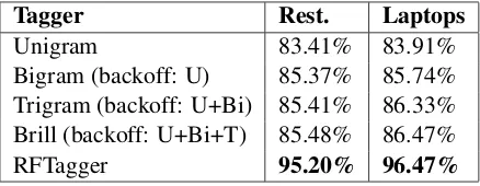
Tagger Rest. Laptops

Unigram 83.41% 83.91% Bigram (backoff: U) 85.37% 85.74% Trigram (backoff: U+Bi) 85.41% 86.33% Brill (backoff: U+Bi+T) 85.48% 86.47% RFTagger 95.20% 96.47%

Table 2: Accuracy of different aspect term taggers.

trial data sets. The table shows that the bigram, tri-gram and Brill taggers achieve only marginal im-provements over a simplistic unigram tagger, even when they are combined through back-off linking. The RFTagger achieved by far the best accuracy on both data sets.

4.1 Results and debugging

Our final results for the full aspect term extraction procedure are shown in Table 3.

Score Rest. Laptops

Precision 57.14% 64.54% Recall 39.15% 60.40% F1-Score 46.47% 62.40%

Table 3: Aspect term extraction results.

The huge difference between tagging accuracy achieved in the development phase and the aspect term extraction quality obtained on the SemEval-2014 test set is caused by different factors. First, Table 2 shows the tagging accuracy across all to-kens, not limited to aspect terms. A tagger that works particularly well for many irrelevant tokens (punctuation, verbs, etc.), correctly marking them ATX, may achieve high accuracy even if it has low recall on tokens belonging to aspect terms. Sec-ond, the official scores only consider an aspect term candidate to be a true positive if it covers exactly the same tokens as the gold standard an-notation. If the tagger disagrees with the human annotators on whether an adjective or determiner should be considered part of an aspect term, this will be counted as a mistake despite the overlap. Thus, even a relatively small number of tagging mistakes near aspect term boundaries will be pun-ished severly in the evaluation. Unseen words as well as long or unusual noun phrases turned out to be particularly difficult.

Table 3 indicates a serious problem with the restaurant data, which has surprisingly low recall,

resulting in an F1-score almost 16 percent points

lower than for the laptop data. A careful exami-nation of the trial, training and test data revealed an early mistake in the preprocessing code as the main culprit. Once this mistake was corrected, the recall score for restaurants was similar to the score for laptops.

5 Aspect term polarity

Subtask 2 is concerned with opinion sentences, i.e. sentences that contain one or more aspect terms and express subjective opinions about (some of) these aspects. Such opinions are expressed through opinion words; common opinion words with their corresponding confidence values (nu-meric values from 1 to 6 expressing the level of certainty that a word is positive or negative, cf. Sec. 2) are collected in sentiment lexica.

The preprocessing stage in this subtask starts with a sentence segmentation step that uses the output of the Stanford CoreNLP parser.3 _All

de-pendencies map onto a directed graph represen-tation where words of each sentence are nodes in the graph and grammatical relations are edge labels. All aspect terms (Sec. 2) are marked in each dependency graph. When processing such a graph we extract all positive and negative opinion words occurring in each sentence by comparing them with word lists contained in our sentiment lexica. A corresponding confidence value from lexica is assigned for each opinion word, the num-ber of positive and negative aspect terms occurring in each sentence are counted and their confidence values are summed up. These values serve as fea-tures for supervised machine learning using algo-rithms implemented in scikit-learn (Pedregosa et al., 2011).

All opinion words that build a dependency with an aspect term are stored for each sentence. A dominant word of each dependency is stored as a governor, whereas a subordinate one is stored as a dependent. Both direct and indirect dependencies are processed. If there are several indirect depen-dencies to an aspect term, they are processed re-cursively. Using lists of extracted dependencies between opinion words and aspect terms hand-writen rules assign corresponding confidence val-ues to aspect terms.

5.1 Features based on a sentiment lexica

The extended sentiment dictionaries were used to extract five features: I) tokens expressing a pos-itive sentiment belonging to one aspect term, II) tokens expressing a negative sentiment, III) con-fidence values of positive tokens, IV) concon-fidence values of negative tokens, V) a sum of all confi-dence values for all positive and all negative opin-ion words occurring in a sentence.

5.2 Features based on hand-written rules

We made use of direct and indirect negation mark-ers, so that all opinion words belonging to a negated aspect term swap their polarity signs. We added rules for negative particlesnotandno that directly precede an opinion word, for adverbs barely, scarcely and too, for such constructions as could have been and wish in the subjunctive mood. After swapping polarity signs of opinion words, a general set of hand-written rules was ap-plied to the graph dependencies. The rules fol-low the order of importance of dependencies scal-ing from least important up to most important. We placed the dependencies in the following or-der: acomp,advmod,nsubjpass,conj and,amod, prep of, prep worth, prep on, prep in, nsubj, inf-mod,dobj,xcomp,rcmod,conj or,appos. All de-pendencies can be grouped into three categories based on the direction of the polarity assignment. The first group (acomp, advmod, amod, rcmod, prep in) includes dependencies where a governor of a dependency takes over polarity of a dependent if the latter is defined. The second group (infmod, conj or, prep on, prep worth, prep of, conj and) covers dependencies in which a dependent ele-ment takes over polarity of a governor if the lat-ter is defined. The third group (dobj, xcomp) is for cases when both governor and dependent are defined. Here a governor takes over polarity of a dependent.

5.3 Experiments

In this section we compare two approches to as-pect term polarity detection. The first approach simply counts all positive and negative words in each sentence and then assigns a label based on which of the two counts is larger. It does not make use of machine learning techniques and its accu-racy is only about 54%. Results improve signifi-cantly with supervised machine learning based on the feature sets described above. We experimented

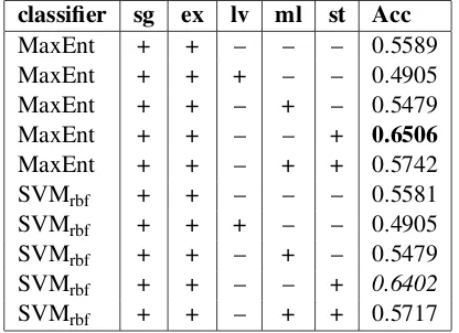
with different classifiers (Maximum Entropy, Lin-ear SVM and SVMs with RBF kernel) and var-ious subsets of features. By default, we worked on the level of single opinion words that express a positive or negative polarity (sg). We added the following features in different combinations: an extended list of opinion words (ex) obtained from a distribution semantic model, based on near-est neighbours of known opinion words (Proisl et al., 2013); potential misspellings of know opin-ion words, within a maximal Levenshtein distance of 1 (lv); word combinations and fixed phrases (ml) containing up to 3 words (e.g., good man-nered, put forth, tried and true, up and down); and the sums of positive and negative opinion words in the whole sentence (st). The best results for the laptops data were achieved with a Max-imum Entropy classifier, excluding misspellings (lv) and word combinations (ml); the correspond-ing line in Table 4 is highlighted in bold font. Even though MaxEnt achieved the best results dur-ing development, we decided to use SVM with a RBF kernel for the test set, assuming that it would be able to exploit interdependencies between fea-tures. The accuracy achieved by the submitted system is highlighted in italics in the table. The training test data provided for restaurants and lap-tops categories were split equally into two sets where the first set (first half) was used for training a model and the second set was used for the test and evaluation stages. Experiments on the restau-rants data produced similar results.

classifier sg ex lv ml st Acc

MaxEnt + + – – – 0.5589 MaxEnt + + + – – 0.4905 MaxEnt + + – + – 0.5479 MaxEnt + + – – + 0.6506

MaxEnt + + – + + 0.5742 SVMrbf + + – – – 0.5581

SVMrbf + + + – – 0.4905

SVMrbf + + – + – 0.5479

SVMrbf + + – – + 0.6402

SVMrbf + + – + + 0.5717

Table 4: Results for laptops category on train set.

6 Aspect category detection

independent parts – one based on machine learn-ing, the other on similarities between WordNet synsets (“synonym sets”, roughly corresponding to concepts). While both approaches achieved similar performance during development, combin-ing them resulted in overall better scores. How-ever, the success of this method crucially depends on accurate indentification of aspect terms.

6.1 A WordNet-based approach4

The WordNet-based component operates on previ-ously identified aspect terms (from the gold stan-dard in the evaluation, but from the module de-scribed in Sec. 4 in a real application setting). For each term, it finds all synsets and compares them to a list of “key synsets” that characterize the different aspect categories (e.g. the category foodis characterized by the key synsetmeal.n.01, among others). The best match is chosen and added to an internal lexicon, which maps each unique phrase appearing as an aspect term to ex-actly one aspect category. As a similarity measure for synsets we used path similarity, which deter-mines the length of the shortest path between two synsets in the WordNet hypernym/hyponym tax-onomy. Key synsets were extracted from a list of high frequency terms and tested manually to cre-ate an accurcre-ate represenation for each ccre-ategory.

In the combined approach this component was taken as a foundation and was augmented by high-confidence suggestions from the machine learning component (see below).

Additional extensions include a high-confidence lexicon based on nearest neighbours from a distributional semantic model, a rudi-mentary lexicon of international dishes, and the application of a spellchecker; together, they accounted only for a small increase in F-score on the development data (from 0.758 to 0.768).

6.2 A machine learning approach5

The machine learning component is essentially a basic bag-of-words model. It employs a multino-mial Naive Bayes classifier in a one-vs-all setup to achieve multi-label classification. In addition to tuning of the smoothing parameters, a probabil-ity threshold was introduced that every predicted category has to pass to be assigned to a sentence.

4_{We used the version of WordNet included in NLTK 2.0.4}

(Bird et al., 2009), accessed through the NLTK API.

5_{We used machine learning algorithms implemented in}

scikit-learn 0.14.1 (Pedregosa et al., 2011).

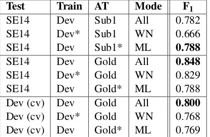
Test Train AT Mode F1

SE14 Dev Sub1 All 0.782 SE14 Dev* Sub1 WN 0.666 SE14 Dev Sub1* ML 0.788

SE14 Dev Gold All 0.848

SE14 Dev* Gold WN 0.829 SE14 Dev Gold* ML 0.788 Dev (cv) Dev Gold All 0.800

Dev (cv) Dev* Gold WN 0.768 Dev (cv) Dev Gold* ML 0.769 *indicates data sets not used by a given component

Table 5: Aspect category detection results.

Different thresholds were used for the stand-alone component (th =0.625) and the combined ap-proach (th=0.9). In the latter case all predici-tions of the WordNet-based component were ac-cepted, but only high-confidence predictions from the Naive Bayes classifier were added.

6.3 Results

Table 5 summarizes the results of different exper-iments with aspect category detection. In all cases the training data consisted of the combined official train and trial sets (Dev). The last three rows show results obtained by ten-fold cross-validation in the development phase, the other rows show the cor-responding results on the official test set (SE14). The first three rows are based on automatically de-tected aspect terms from the module described in Sec. 4 (Sub 1), the other rows used gold standard aspect terms. Separate results are provided for the combined approach (Mode: All) as well as for the two individual components (WN = WordNet, ML = machine learning). Note that the WN compo-nent does not require any training data, while the ML component does not make use of aspect terms marked in the input.

Bayes bag-of-words model.

7 Aspect category polarity

The general approach was to allocate each aspect term to the corresponding aspect categories. A simple rule set was then used to determine the po-larity of each aspect category based on the polari-ties of the aligned aspect terms. In cases where no aspect terms are marked (but sentences are still la-belled with aspect categories), the idea was to fall back on the sentiment values for the entire sen-tences provided by the CoreNLP suite.6

7.1 Term / category alignment

To establish a basis for creating the mapping rules, the first step was to work out the distribution of aspect terms and aspect categories in the train-ing data. The most common case is that an as-pect category aligns with a single asas-pect term (1476×); there are also many aspect categories with multiple aspect terms (1179×) and some as-pect categories without any asas-pect terms. Since the WordNet-Approach from Sec. 6 showed rela-tively good results (especially if gold standard as-pect terms are available, which is the case here), a modified version was used to assign each aspect term to one of the annotated categories.

7.2 Polarity allocation

After the assignment of aspect terms to their ac-cording aspect category – if needed – the aspect category polarity can be determined. For this, the polarity values of all aspect terms assigned to this category were collected, and duplicates were re-moved in order to produce a unique set (e.g. 1, 1, -1, 0, 0 would be reduced to 1, -1, 0). A set with both negative and positive polarity values in-dicates a conflict for the corresponding aspect cat-egory, while a neutral polarity value would be ig-nored, if positive or negative polarity values occur. Our method achieved an accuracy of 89.16% for sentences annotated with just a single aspect cat-egory. In cases where only one aspect term had been assigned to a aspect category the accuracy was unsuprisingly high (96.61%), whereas the ac-curacy decreased in cases of multiple assigned as-pect terms (78.44%). For asas-pect categories with-out aligned aspect terms, as well as the category anecdotes/miscellaneous, the sentiment values of the CoreNLP sentiment analysis tool had to be

6_{http://nlp.stanford.edu/software/corenlp.shtml}

used, which led to a poor accuracy in those cases, namely 52.74%.

7.3 Results

On the official test set, the module for subtask 4 achieved an accuracy of 69.56%. An important factor is the very low accuracy in cases where the CoreNLP sentiment value for the entire sentence had to be used. We expect a considerable improve-ment from using a modified version of the subtask 2 module (Sec. 5) to compute overall sentence po-larity.

8 Conclusion

We have shown a modular system working as a pipeline that modifies the input sentences step by step by adding new information as XML tags. Aspect term extraction was handled as a tagging task that utilized an IOB tagset to find aspect terms with the final version relying on Schmid’s RFTagger. Determination of aspect term polar-ity was achieved through a machine learning ap-proach that uses SVMs with RBF kernel. This was supported by an augmented sentiment lexicon based on several different sources, which was ex-panded manually by a team of students. Aspect category detection in turn employs a combination approach of an algorithm depending on WordNet synsets and a bag-of-words Naive Bayes classifier. Finally aspect category polarity was calculated by combining the results from the last two modules.

Overall results were satisfactory, being mostly in the top half of submitted systems. During phase A of testing (subtasks 1 and 3), a preprocessing er-ror caused a massive drop in performance in aspect term extraction. This carried over to the other sub-task, because the module uses aspect terms among other features to identify aspect categories. Scores for phase B (subtasks 2 and 4) were very close to test results during development with the exception of cases where the CoreNLP sentiment value for an entire sentence had to be used.

References

Steven Bird, Ewan Klein, and Edward Loper. 2009. Natural Language Processing with Python. O’Reilly Media.

Minqing Hu and Bing Liu. 2004. Mining and summa-rizing customer reviews. InProceedings of the 10th ACM SIGKDD International Conference on Knowl-edge Discovery and Data Mining (KDD ’04), pages 168–177, Seattle, WA.

Finn ˚Arup Nielsen. 2011. A new ANEW: Evaluation of a word list for sentiment analysis in microblogs. InProceedings of the ESWC2011 Workshop on Mak-ing Sense of Microposts: Big thMak-ings come in small packages, number 718 in CEUR Workshop Proceed-ings, pages 93–98, Heraklion, Greece, May. Fabian Pedregosa, Ga¨el Varoquaux, Alexandre

Gram-fort, Vincent Michel, Bertrand Thirion, Olivier Grisel, Mathieu Blondel, Peter Prettenhofer, Ron Weiss, Vincent Dubourg, Jake Vanderplas, Alexan-dre Passos, David Cournapeau, Matthieu Brucher, Matthieu Perrot, and ´Edouard Duchesnay. 2011. Scikit-learn: Machine learning in Python. Journal of Machine Learning Research, 12:2825–2830. Maria Pontiki, Dimitrios Galanis, John

Pavlopou-los, Harris Papageorgiou, Ion AndroutsopouPavlopou-los, and Suresh Manandhar. 2014. SemEval-2014 task 4: Aspect based sentiment analysis. InProceedings of the 8th International Workshop on Semantic Evalu-ation (SemEval 2014), Dublin, Ireland.

Thomas Proisl, Paul Greiner, Stefan Evert, and Besim Kabashi. 2013. KLUE: Simple and robust meth-ods for polarity classification. In Second Joint Conference on Lexical and Computational Seman-tics (*SEM), Volume 2: Proceedings of the Sev-enth International Workshop on Semantic Evalua-tion (SemEval 2013), pages 395–401, Atlanta, Geor-gia, USA, June. Association for Computational Lin-guistics.

Helmut Schmid and Florian Laws. 2008. Estimation of conditional probabilities with decision trees and an application to fine-grained POS tagging. In Pro-ceedings of the 22nd International Conference on Computational Linguistics, volume 1, pages 777– 784.