Minimum Risk Training of Approximate CRF Based NLP Systems

Minimum-Risk Training of Approximate CRF-Based NLP Systems

Veselin Stoyanov and Jason Eisner

HLTCOE and Center for Language and Speech Processing Johns Hopkins University

Baltimore, MD 21218 {ves, jason}@cs.jhu.edu

Abstract

Conditional Random Fields (CRFs) are a pop-ular formalism for structured prediction in NLP. It is well known how to train CRFs with certain topologies that admit exact inference, such as linear-chain CRFs. Some NLP phe-nomena, however, suggest CRFs with more complex topologies. Should such models be used, considering that they make exact infer-ence intractable? Stoyanov et al. (2011) re-cently argued for training parameters to min-imize the task-specific loss of whatever ap-proximate inference and decoding methods will be used at test time. We apply their method to three NLP problems, showing that (i) using more complex CRFs leads to im-proved performance, and that (ii) minimum-risk training learns more accurate models.

1 Introduction

Conditional Random Fields (CRFs) (Lafferty et al., 2001) are often used to model dependencies among linguistic variables. CRF-based models have im-proved the state of the art in a number of natural language processing (NLP) tasks ranging from part-of-speech tagging to information extraction and sen-timent analysis (Lafferty et al., 2001; Peng and Mc-Callum, 2006; Choi et al., 2005).

Robust and theoretically sound training proce-dures have been developed for CRFs when the model can be used with exact inference and de-coding.1 However, some NLP problems seem to

1_{“Inference” typically refers to computing posterior} marginal or max-marginal probability distributions of output random variables, given some evidence. “Decoding” derives a single structured output from the results of inference.

call for higher-treewidth graphical models in which exact inference is expensive or intractable. These “loopy” CRFs have cyclic connections among the output and/or latent variables. Alas, standard learn-ing procedures assume exact inference: they do not compensate for approximations that will be used at test time, and can go surprisingly awry if approxi-mate inference is used at training time (Kulesza and Pereira, 2008).

While NLP research has been consistently evolv-ing toward more richly structured models, one may hesitate to add dependencies to a graphical model if there is a danger that this will end uphurting per-formance through approximations. In this paper we illustrate how to address this problem, even for ex-tremely interconnected models in which every pair of output variables is connected.

Wainwright (2006) showed that if approximate in-ference will be used at test time, it may be beneficial to use a learning procedure that does not converge to the true model but to one that performs wellunder the approximations. Stoyanov et al. (2011) argue for minimizing a certain non-convex training objective, namely the empirical risk of the entire system com-prising the CRFtogetherwith whatever approximate inference and decoding procedures will be used at test time. They regard this entire system as sim-ply a complex decision rule, analogous to a neu-ral network, and show how to use back-propagation to tune its parameters to locally minimize the em-pirical risk (i.e., the average task-specific loss on training data). Stoyanov et al. (2011) show that on certain synthetic-dataproblems, this frequentist training regimen significantly reduced test-data loss

compared to approximate maximum likelihood esti-mation (MLE). However, this method has not been evaluated onreal-worldproblems until now.

We will refer to the Stoyanov et al. (2011) ap-proach as “ERMA”—Empirical Risk Minimization under Approximations. ERMA is attractive for NLP because the freedom to use arbitrarily structured graphical models makes it possible to include latent linguistic variables, predict complex structures such as parses (Smith and Eisner, 2008), and do collec-tive prediction in relational domains (Ji and Grish-man, 2011; Benson et al., 2011; Dreyer and Eis-ner, 2009). In training, ERMA considers not only the approximation method but also the task-specific loss function. This means that ERMA is careful to use the additional variables and dependencies only in ways that help training set performance. (Overfit-ting on the enlarged parameter set should be avoided through regularization.)

We have developed a simple syntax for specify-ing CRFs with complex structures, and a software package (available from http://www.clsp.

jhu.edu/˜ves/software.html) that allows

ERMA training of these CRFs for several popular loss functions (e.g., accuracy, mean-squared error, F-measure). In this paper, we use these tools to re-visit three previously studied NLP applications that can be modeled naturally with approximate CRFs (we will useapproximate CRFs to refer to CRF-based systems that are used with approximations in inference or decoding). We show that (i) natural lan-guage can be modeled more effectively with CRFs that are not restricted to a linear structure and (ii) that ERMA training represents an improvement over previous learning methods.

The first application, predicting congressional votes, has not been previously modeled with CRFs. By using a more principled probabilistic approach, we are able to improve the state-of-the-art accuracy from 71.2% to 78.2% when training to maximize the approximate log-likelihood of the training data. By switching to ERMA training, we improve this result further to 85.1%.

The second application, information extraction from seminar announcements, has been modeled previously with skip-chain CRFs (Sutton and Mc-Callum, 2005; Finkel et al., 2005). The skip-chain CRF introduces loops and requires approximate

in-ference, which motivates minimum risk training. Our results show that ERMA training improves F-measures from 89.5 to 90.9 (compared to 87.1 for the model without skip-chains).

Finally, for our third application, we perform col-lective multi-label text classification. We follow pre-vious work (Ghamrawi and McCallum, 2005; Finley and Joachims, 2008) and use a fully connected CRF to model all pairwise dependencies between labels. We observe similar trends for this task: switching from a maximum entropy model that does not model label dependencies to a loopy CRF leads to an im-provement in F-measure from 81.6 to 84.0, and us-ing ERMA leads to additional improvement (84.7).

2 Preliminaries

2.1 Conditional Random Fields

Aconditional random field(CRF) is an undirected graphical model defined by a tuple(X,Y,F, f, θ).

X = (X1, X2, . . .)is a set of random variables and Y = (Y1, Y2, . . .) is a set of output random

vari-ables.2 We usex= (x1, x2, . . .), to denote a

possi-ble assignment of values toX, and similarly for y, withxydenoting the joint assignment. Eachα∈ F

is a subset of the random variables, α ⊆ X ∪ Y, and we writexy_αto denote the restriction ofxyto α. Finally, for each α ∈ F, the CRF specifies a functionf~αthat extracts a feature vector∈Rdfrom

the restricted assignmentxy_α. We define the over-all feature vectorf~(x,y) = P

α∈Ff~α(xyα) ∈Rd.

The model defines conditional probabilities

pθ(y|x) =

exp~θ·f~(x,y) P

y0exp~θ·f~(x,y0)

(1)

where θ~ ∈ Rd is a global weight vector (to be

learned). This is a log-linear model; the denomina-tor (traditionally denotedZx) sums over all possible output assignments to normalize the distribution.

Provided that all probabilities needed at training or test time are conditioned on an observation of the formX = x, CRFs can include arbitrary overlap-ping features of the input without having to explic-itly model input feature dependencies.

2

2.2 Inference in CRFs

Inference in general CRFs is intractable (Koller and Friedman, 2009). Nevertheless, there exist several approximate algorithms that have theoretical moti-vation and tend to exhibit good performance in prac-tice. Those include variational methods such as loopy belief propagation (BP) (Murphy et al., 1999) and mean-field, as well as Markov Chain Monte Carlo methods.

ERMA training is applicable to any approxima-tion that corresponds to a differentiable funcapproxima-tion, even if the function has no simple closed form but is computed by an iterative update algorithm. In this paper we select BP, which is exact when the fac-tor graph is a tree, such as a linear-chain CRF, but whose results can be somewhat distorted by loops in the factor graph, as in our settings. BP computes beliefs about the marginal distribution of each ran-dom variable using iterative updates. We standardly approximate theposteriorCRF marginals given the input observations by running BP over a CRF that enforces those observations.

2.3 Decoding

Conditional random fields are models of probabil-ity. A decoder is a procedure for converting these probabilities into system outputs. Givenx, the de-coder would ideally choose yto minimize the loss `(y,y∗), where`compares a candidate assignment

yto the true assignmenty∗. But of course we do not know the truth at test time. Instead we can average overpossiblevaluesy0of the truth:

argmin

y

X

y0

p(y0 |x)·`(y,y0) (2)

This is the minimum Bayes risk (MBR)principle from statistical decision theory: choose yto mini-mize the expected loss (i.e., the risk) according to the CRF’s posterior beliefs givenx.

In the NLP literature, CRFs are often decoded by choosing yto be the maximum posterior probabil-ity assignment (e.g., Sha and Pereira (2003), Sutton et al. (2007)). This is the MBR procedure for the 0-1 loss function that simply tests whethery =y∗. For other loss functions, however, the corresponding MBR procedure is preferable. For some loss func-tions it is tractable given the posterior marginals of p, while in other cases approximations are needed.

In our experiments we use MBR decoding (or a tractable approximation) but substitute the approx-imate posterior marginals ofpas computed by BP. For example, if the loss ofyis the number of incor-rectly recovered output variables, MBR says to sep-arately pick the most probable value for each output variable, according to its (approximate) marginal.

3 Minimum-Risk CRF Training

This section briefly describes the ERMA training al-gorithm from Stoyanov et al. (2011) and compares it to related structured learning methods. We assume a standard ML setting, with a set of training inputs

xi and corresponding correct outputs yi∗. All the methods below are regularized in practice, but we omit mention of regularizers for simplicity.

3.1 Related Structured Learning Methods

When inference and decoding can be performed ex-actly, the CRF parameters ~θ are often trained by maximum likelihood estimation (MLE):

argmax θ

X

i

logpθ(yi∗ |xi) (3)

The gradient of each summand logpθ(yi∗ | xi)

than each possible alternative yi ∈ Y. The loss is incorporated in these methods by requiring the mar-gin(~θ·f~(xi_,yi∗_{)−~θ·f~(x}i_,yi_))≥`(yi_,yi∗_{), with}

penalized slack in these constraints. The softmax-margin method uses a different criterion—it resem-bles MLE but modifies the denominator of (1) to Zx=P_y0_∈Yexp(θ~·f~(x,y0) +`(y0,y∗)).

In our experiments we compare against MLE training (which is common) and softmax-margin, which incorporates loss and which Gimpel and Smith (2010) show is either better or competitive when compared to other margin methods on an NLP task. We adapt these methods to the loopy case in the obvious way, by replacing exact inference with loopy BP and keeping everything else the same.

3.2 Minimum-Risk Training

We wish to consider the approximate inference and decoding algorithms and the loss function that will be used during testing. Thus, we wantθto minimize the expected loss under the true data distributionP:

argmin θ

Exy∼P[`(δθ(x),y)] (4)

whereδθ is the decision rule (parameterized by θ),

which decodes the results of inference underpθ.

In practice, we do not know the true data distri-bution, but we can doempirical risk minimization (ERM), instead averaging the loss over our sample of(xi_,yi_{)pairs. ERM for structured prediction was}

first introduced in the speech community (Bahl et al., 1988) and later used in NLP (Och, 2003; Kakade et al., 2002; Suzuki et al., 2006; Li and Eisner, 2009, etc.). Previous applications of risk minimization as-sumeexact inference, having defined the hypothe-sis space by a precomputed n-best list, lattice, or packed forest over which exact inference is possible. The ERMA approach (Stoyanov et al., 2011) works with approximate inference and computes ex-act gradients of the output loss (or a differentiable surrogate) in the context of the approximate infer-ence and decoding algorithms. To determine the gra-dient of`(δθ(xi),yi)with respect to θ, the method

relies on automatic differentiation in the reverse mode (Griewank and Corliss, 1991), a general tech-nique for sensitivity analysis in computations. The intuition behind automatic differentiation is that the

entire computation is a sequence of elementary dif-ferentiable operations. For each elementary opera-tion, given that we know the input and result values, and the partial derivative of the loss with respect to the result, we can compute the partial derivative of the loss with respect to the inputs to the step. Dif-ferentiating the whole complicated computation can be carried out in backward pass in this step-by-step manner as long as we record intermediate results during the computation of the function (the forward pass). At the end, we accumulate the partials of the loss with respect to each parameterθi.

ERMA is similar to back-propagation used in re-current neural networks, which involve cyclic up-dates like those in belief propagation (Williams and Zipser, 1989). It considers an “unrolled” version of the forward pass, in which “snapshots” of a vari-able at timestandt+ 1are treated as distinct vari-ables, with one perhaps influencing the other. The forward pass computes`(δθ(xi),yi)by performing

approximate inference, then decoding, then evalu-ation. These steps convert(xi, θ) → marginals →

decision→loss. The backward pass rewinds the en-tire computation, differentiating each phase in term. The total time required by this algorithm is roughly twice the time of the forward pass, so its complexity is comparable to approximate inference.

We gradually reduce the temperatureT ∈_Rfrom 1 to 0 as training proceeds, which turns sum-product inference into max-product by moving all the prob-ability mass toward the highest-scoring assignment.

4 Modeling Natural Language with CRFs

This section describes three NLP problems that can be naturally modeled with approximate CRFs. The first problem, modeling congressional votes, has not been previously modeled with a CRF. We show that by switching to the principled CRF framework we can learn models that are much more accurate when evaluated on test data, though using the same (or less expressive) features as previous work. The other two problems, information extraction from semi-structured text and collective multi-label classifica-tion, have been modeled with loopy CRFs before. For all three models, we show that ERMA training results in better test set performance.3

4.1 Modeling Congressional Votes

The Congressional Vote (ConVote) corpus was cre-ated by Thomas et al. (2006) to study whether votes of U.S. congressional representatives can be pre-dicted from the speeches they gave when debating a bill. The corpus consists of transcripts of con-gressional floor debates split into speech segments. Each speech segment is labeled with the represen-tative who is speaking and the recorded vote of that representative on the bill. We aim to predict a high percentage of the recorded votes correctly.

Speakers often reference one another (e.g., “I thank the gentleman from Utah”), to indicate agree-ment or disagreeagree-ment. The ConVote corpus manu-ally annotates each phrase such as “the gentleman from Utah” with the representative that it denotes.

Thomas et al. (2006) show that classification us-ing the agreement/disagreement information in the local context of such references, together with the rest of the language in the speeches, can lead to sig-nificant improvement over using either of these two

3_{We also experimented with a fourth application, joint POS} tagging and shallow parsing (Sutton et al., 2007) and observed the same overall trend (i.e., minimum risk training improved performance significantly). We do not include those experi-ments, however, because we were unable to make our baseline results replicate (Sutton et al., 2007).

sources of information in isolation. The original ap-proach of Thomas et al. (2006) is based on training two Support Vector Machine (SVM) classifiers— one for classifying speeches as supporting/opposing the legislation and another for classifying references as agreement/disagreement. Both classifiers rely on bag-of-word (unigram) features of the document and the context surrounding the link respectively. The scores produced by the two SVMs are used to weight a global graph whose vertices are the representa-tives; then the min-cut algorithm is applied to par-tition the vertices into “yea” and “nay” voters.

While the approach of Thomas et al. (2006) leads to significant improvement over using the first SVM alone, it does not admit a probabilistic in-terpretation and the two classifiers are not trained jointly. We also remark that the min-cut technique would not generalize beyond binary random vari-ables (yea/nay).

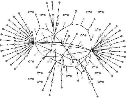
We observe that congressional votes together with references between speakers can be naturally mod-eled with a CRF. Figure 1 depicts the CRF con-structed for one of the debates in the development part of the ConVote corpus. It contains a random variable for each representative’s vote. In addition, each speech is an observed input random variable: it is connected by a factor to its speaker’s vote and encourages it to be “yea” or “nay” according to fea-tures of the text of the speech. Finally, each ref-erence in each speech is an observed input random variable connected by a factor to two votes—those of the speaker and the referent—which it encourages to agree or disagree according to features of the text surrounding the reference. Just as in (Thomas et al., 2006), the score of a global assignment to all votes is defined by considering both kinds of factors. How-ever, unlike min-cut, CRF inference finds a proba-bility distribution over assignments, not just a sin-gle best assignment. This fact allows us to train the two kinds of factors jointly (on the set of training debates where the votes are known) to predict the correct votes accurately (as defined by accuracy).

Figure 1: An example of a debate structure from the Con-Vote corpus. Each black square node represents a factor and is connected to the variables in that factor, shown as round nodes. Unshaded variables correspond to the representatives’ votes and depict the output variables that we learn to jointly predict. Shaded variables correspond to the observed input data— the text of all speeches of a representative (in dark gray) or all local contexts of refer-ences between two representatives (in light gray).

and that ERMA further significantly improves per-formance, particularly when it properly trains with the same inference algorithm (max-product vs. sum-product) to be used at test time.

Baseline. As an exact baseline, we compare against the results of Thomas et al. (2006). Their test-time Min-Cut algorithm is exact in this case: bi-nary variables and a two-way classification.

4.2 Information Extraction from Semi-Structured Text

We utilize the CMU seminar announcement corpus of Freitag (2000) consisting of emails with seminar announcements. The task is to extract four fields that describe each seminar: speaker, location, start time

andend time. The corpus annotates the document with all mentions of these four fields.

Sequential CRFs have been used successfully for semi-structured information extraction (Sutton and McCallum, 2005; Finkel et al., 2005). However, they cannot model non-local dependencies in the data. For example, in the seminar announcements corpus, if “Sutner” is mentioned once in an email in a context that identifies him as a speaker, it is

Sutner

S

Who:

O

Prof.

S

Klaus

S

will

O

Prof.

S

Sutner

S

… …

… …

Figure 2: Skip-chain CRF for semi-structured informa-tion extracinforma-tion.

likely that other occurrences of “Sutner” in the same email should be marked asspeaker. Hence Finkel et al. (2005) and Sutton and McCallum (2005) propose adding non-local edges to a sequential CRF to repre-sent soft consistency constraints. The model, called a “skip-chain CRF” and shown in Figure 2, contains a factor linking each pair of capitalized words with the same lexical form. The skip-chain CRF model exhibits better empirical performance than its se-quential counterpart (Sutton and McCallum, 2005; Finkel et al., 2005).

The non-local skip links make exact inference intractable. To train the full model, Finkel et al. (2005) estimate the parameters of a sequential CRF and then manually select values for the weights of the non-local edges. At test time, they use Gibbs sampling to perform inference. Sutton and McCal-lum (2005) use max-product loopy belief propaga-tion for test-time inference, and compare a train-ing procedure that uses a piecewise approximation of the partition function against using sum-product loopy belief propagation to compute output variable marginals. They find that the two training regimens perform similarly on the overall task. All of these training procedures try to approximately maximize conditional likelihood, whereas we will aim to mini-mize the empirical loss of the approximate inference and decoding procedures.

Baseline. As an exact (non-loopy) baseline, we train a model without the skip chains. We give two baseline numbers in Table 1—for training the exact CRF with MLE and with ERM. The ERM setting re-sulted in a statistically significant improvement even in the exact case, thanks to the use of the loss func-tion at training time.

4.3 Multi-Label Classification

war.” The most straightforward approach to multi-label classification employs a binary classifier for each class separately. However, previous work has shown that incorporating information about label de-pendencies can lead to improvement in performance (Elisseeff and Weston, 2001; Ghamrawi and McCal-lum, 2005; Finley and Joachims, 2008).

For this task we follow Ghamrawi and McCallum (2005) and Finley and Joachims (2008) and model the label interactions by constructing a fully con-nected CRF between the output labels. That is, for every document, we construct a CRF that contains a binary random variable for each label (indicating that the corresponding label is on/off for the doc-ument) and one binary edge for every unique pair of labels. This architecture can represent dependen-cies between labels, but leads to a setting in which the output variables form one massive clique. The resulting intractability of inference (and decoding) motivates the use of ERMA training.

Baseline. We train a model without any of the pairwise edges (i.e., a separate logistic regression model for each class). We report the single best baseline number, since MLE and ERM training re-sulted in statistically indistinguishable results.

5 Experiments

5.1 Learning Methodology

For all experiments we split the data into train/development/test sets using the standard splits when available. We tune optimization algorithm pa-rameters (initial learning rate, batch size and meta-parametersλandµfor stochastic meta descent) on the training set based on training objective conver-gence rates. We tune the regularization parameter β(below) on development data when available, oth-erwise we use a default value of 0.1—performance was generally robust for small changes in the value ofβ. All statistical significance testing is performed using paired permutation tests (Good, 2000).

Gradient-based Optimization. Gradient infor-mation from the back-propagation procedure can be used in a local optimization method to minimize em-pirical loss. In this paper we use stochastic meta descent (SMD) (Schraudolph, 1999). SMD is a second-order method that requires vector-Hessian

products. For computing those, we do not need to maintain the full Hessian matrix. Instead, we apply more automatic differentiation magic—this time in the forward mode. Computing the vector-Hessian product and utilizing it in SMD does not add to the asymptotic runtime, it requires about twice as many arithmetic operations, and leads to much faster con-vergence of the learner in our experience. See Stoy-anov et al. (2011) for details.

Since the empirical risk objective could overfit the training data, we add anL2regularizerβP_jθj2

that prefers parameter values close to 0. This im-proves generalization, like the margin constraints in margin-based methods.

Training Procedure Stoyanov et al. (2011) ob-served that the minimum-risk objective tends to be highly non-convex in practice. The usual approx-imate log likelihood training objective appeared to be smoother over the parameter space, but exhibited global maxima at parameter values that were rela-tively good, but sub-optimal for other loss functions. Mean-squared error (MSE) also gave a smoother ob-jective than other loss functions. These observations motivated Stoyanov et al. (2011) to use a contin-uation method. They optimized approximate log-likelihood for a few iterations to get to a good part of the parameter space, then switched to using the hy-brid loss functionλ`(y, y0)+(1−λ)`MSE(y, y0). The coefficientλchanged gradually from0 to1during training, which morphs from optimizing a smoother loss to optimizing the desired bumpy test loss. We follow the same procedure.

Experiments in this paper use two evaluation met-rics: percentage accuracy and F-measure. For both of these losses we decode by selecting the most probable value under the marginal distribution of each random variable. This is an exact MBR de-code for accuracy but an approximate one for the F-measure; our ERMA training will try to compen-sate for this approximate decoder. This decoding procedure is not differentiable due to the use of the

argmax function. To make the decoder

differen-tiable, we replace argmax with a stochastic (soft-max) version during training, averaging loss over all possible values v in proportion to their exponenti-ated probability p(yi = v | x)1/Tdecode. This

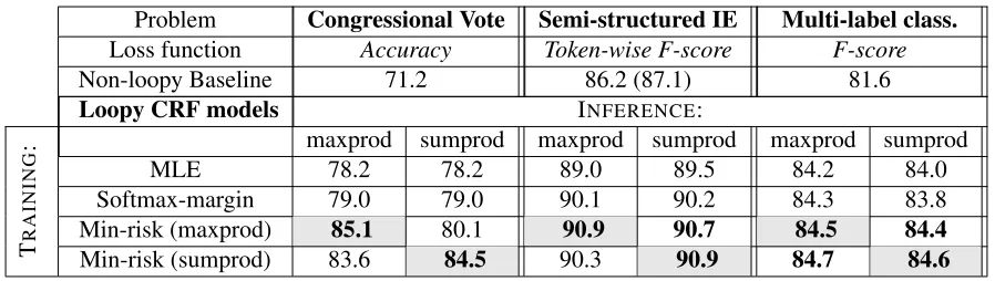
Problem Congressional Vote Semi-structured IE Multi-label class. Loss function Accuracy Token-wise F-score F-score

Non-loopy Baseline 71.2 86.2 (87.1) 81.6

Loopy CRF models INFERENCE:

T

R

A

IN

IN

G

: maxprod sumprod maxprod sumprod maxprod sumprod

MLE 78.2 78.2 89.0 89.5 84.2 84.0

Softmax-margin 79.0 79.0 90.1 90.2 84.3 83.8

Min-risk (maxprod) 85.1 80.1 90.9 90.7 84.5 84.4 Min-risk (sumprod) 83.6 84.5 90.3 90.9 84.7 84.6

Table 1: Results. The top of the table lists the loss function used for each problem and the score for the best exact baseline. The bottom lists results for the full models used with loopy BP. Models are tested with either sum-product BP (sumprod) or max-product BP (maxprod) and trained with MLE or the minimum risk criterion. Min-risk training runs are either annealed (maxprod), which matches max-product test, or not (sumprod), which matches sum-product test; grey cells in the table indicate matched training and test settings. In each column, we boldface the best result as well as all results that are not significantly worse (paired permutation test,p <0.05).

decoder asTdecode decreases toward 0. For simplic-ity, our experiments just use a single fixed value of

0.1forTdecode. Annealing the decoder slowly did not lead to significant differences in early experiments on development data.

5.2 Results

Table 1 lists results of our evaluation. For all three of our problems, using approximate CRFs results in statistically significant improvement over the ex-act baselines, for any of the training procedures. But among the training procedures for approximate CRFs, our ERMA procedure—minimizing empiri-cal risk with the training setting matched to the test setting—improves over the two baselines, namely MLE and softmax-margin. MLE and softmax-margin training were statistically indistinguishable in our experiments with the exception of semi-structured IE. ERMA’s improvements over them are statistically significant at the p < .05 level for the Congressional Vote and Semi-Structured IE prob-lems and at thep < .1level for the Multi-label clas-sification problem (comparing each matched min-risk setting shown in a gray cell in Table 1 vs. MLE). When minimizing risk, we also observe that matching training and test-time procedures can re-sult in improved performance in one of the three problems, Congressional Vote. For this problem, the matched training condition performs better than the alternatives (accuracy of85.1 vs. 83.6 for the an-nealed max-product testing and84.5vs80.1for the

sum-product setting), significant at p < .01). We observe the same effect for semi-structured IE when testing using max-product inference. For the other remaining three problem setting training with either minimal risk training regiment.

Finally, we hypothesized that sum-product infer-ence may produce more accurate results in certain cases as it allows more information about differ-ent parts of the model to be exchanged. How-ever, our results show that for these three problems, sum-product and max-product inference yield statis-tically indistinguishable results. This may be be-cause the particular CRFs we used included no la-tent variables (in constrast to the synthetic CRFs in Stoyanov et al. (2011)). As expected, we found that max-product BP converges in fewer iterations— sum-product BP required as many as twice the num-ber of iterations for some of the runs.

Results in this paper represent a new state-of-the-art for the first two of the problems, Congressional Vote and Semi-structured IE. For Multi-Label classi-fication, comparing against the SVM-based method of Finley and Joachims (2008) goes beyond the scope of this paper.

6 Related Work

tree-shaped or linear chain MRFs and CRFs (Kakade et al., 2002; Suzuki et al., 2006; Gross et al., 2007).

All of the above focus on exact inference. Our approach can be seen as generalizing these methods to arbitrary graph structures, arbitrary loss functions and approximate inference.

Lacoste-Julien et al. (2011) also consider the ef-fects of approximate inference on loss. However, they assume the parameters are given, and modify the approximate inference algorithm at test time to consider the loss function.

Using empirical risk minimization totrain graph-ical models was independently proposed by Domke (2010; 2011). Just as in our own paper (Stoy-anov et al., 2011), Domke took a decision-theoretic stance and proposed ERM as a way of calibrating the graphical model for use with approximate infer-ence, or for use with data that do not quite match the modeling assumptions.4

In particular, (Domke, 2011) is similar to (Stoy-anov et al., 2011) in using ERMA to train model pa-rameters to be used with “truncated” inference that will be run for only a fixed number of iterations. For a common pixel-labeling benchmark in computer vi-sion, Domke (2011) shows that this procedure im-proves training time by orders of magnitude, and slightly improves accuracy if the same number of message-passing iterations is used at test time.

Stoyanov and Eisner (2011) extend the ERMA objective function by adding an explicit runtime term. This allows them to tune model parameters and stopping criteria to learn models that obtain a given speed-accuracy tradeoff. Their approach im-proves this hybrid objective over a range of coeffi-cients when compared to the traditional way of in-ducing sparse structures through L1 regularization.

Eisner and Daum´e III (2011) propose the same lin-ear combination of speed and accuracy as a rein-forcement learning objective. In general, our pro-posed ERMA setting resembles the reinforcement learning problem of trying to directly learn a policy that minimizes loss or maximizes reward.

We have been concerned with the fact that ERMA training objectives may suffer from local optima and non-differentiability. Stoyanov et al. (2011) studied

4

However, he is less focused than we are on matching train-ing conditions to test conditions (by includtrain-ing the decoder and task loss in the ERMA objective).

several such settings, graphed the difficult objective, and identified some practical workarounds that are used in the present paper. Although these methods have enabled us to get strong results by reducing the empirical risk, we suspect that ERMA training ob-jectives will benefit from more sophisticated opti-mization methods. This is true even when the ap-proximate inference itself is restricted to be some-thing as simple as a convex minimization. While that simplified setting can make it slightly more con-venient tocomputethe gradient of the inference re-sult with respect to the parameters (Domke, 2008; Domke, 2012), there is still no guarantee that follow-ing that gradient will minimize the empirical risk. Convex inference does not imply convex training.

7 Conclusions

Motivated by the recently proposed method of Stoy-anov et al. (2011) for minimum-risk training of CRF-based systems, we revisited three NLP do-mains that can naturally be modeled with approx-imate CRF-based systems. These include appli-cations that have not been modeled with CRFs before (the ConVote corpus), as well as applica-tions that have been modeled with loopy CRFs trained to minimize the approximate log-likelihood (semi-structured information extraction and collec-tive multi-label classification). We show that (i) the NLP models are improved by moving to richer CRFs that require approximate inference, and (ii) empirical performance is always significantly im-proved by training to reduce the loss that would be achieved by approximate inference, even compared to another state-of-the-art training method (softmax-margin) that also considers loss and uses approxi-mate inference. The general software package that implements the algorithms in this paper is avail-able at http://www.clsp.jhu.edu/˜ves/

software.html.

Acknowledgments

References

L. Bahl, P. Brown, P. de Souza, and R. Mercer. 1988. A new algorithm for the estimation of hidden Markov model parameters. InProceedings of ICASSP, pages 493–496.

E. Benson, A. Haghighi, and R. Barzilay. 2011. Event discovery in social media feeds. In Proceedings of ACL-HLT, pages 389–398.

Y. Choi, C. Cardie, E. Riloff, and S. Patwardhan. 2005. Identifying sources of opinions with conditional ran-dom fields and extraction patterns. InProceedings of HLT/EMNLP, pages 355–362.

J. Domke. 2008. Learning convex inference of marginals. InProceedings of UAI.

J. Domke. 2010. Implicit differentiation by perturba-tion. In Advances in Neural Information Processing Systems, pages 523–531.

J. Domke. 2011. Parameter learning with truncated message-passing. In Proceedings of the IEEE Con-ference on Computer Vision and Pattern Recognition (CVPR).

J. Domke. 2012. Generic methods for optimization-based modeling. InProceedings of AISTATS.

M. Dreyer and J. Eisner. 2009. Graphical models over multiple strings. In Proceedings of EMNLP, pages 101–110.

J. Eisner and Hal Daum´e III. 2011. Learning speed-accuracy tradeoffs in nondeterministic inference al-gorithms. In COST: NIPS 2011 Workshop on Com-putational Trade-offs in Statistical Learning, Sierra Nevada, Spain, December.

A. Elisseeff and J. Weston. 2001. Kernel methods for multi-labelled classification and categorical regression problems. In Advances in Neural Information Pro-cessing Systems, pages 681–687.

J.R. Finkel, T. Grenager, and C. Manning. 2005. In-corporating non-local information into information ex-traction systems by Gibbs sampling. InProceedings of ACL, pages 363–370.

T. Finley and T. Joachims. 2008. Training structural SVMs when exact inference is intractable. In Proceed-ings of ICML, pages 304–311.

D. Freitag. 2000. Machine learning for information extraction in informal domains. Machine learning, 39(2).

N. Ghamrawi and A. McCallum. 2005. Collective multi-label classification. In Proceedings of CIKM, pages 195–200.

K. Gimpel and N.A. Smith. 2010. Softmax-margin CRFs: Training log-linear models with cost functions. InProceedings of ACL, pages 733–736.

P. I. Good. 2000.Permutation Tests. Springer.

A. Griewank and G. Corliss, editors. 1991. Automatic Differentiation of Algorithms. SIAM, Philadelphia. S. Gross, O. Russakovsky, C. Do, and S. Batzoglou.

2007. Training conditional random fields for maxi-mum labelwise accuracy. Advances in Neural Infor-mation Processing Systems, 19:529.

H. Ji and R. Grishman. 2011. Knowledge base popula-tion: Successful approaches and challenges. In Pro-ceedings of ACL-HLT, pages 1148–1158.

S. Kakade, Y.W. Teh, and S. Roweis. 2002. An alternate objective function for Markovian fields. In Proceed-ings of ICML, pages 275–282.

D. Koller and N. Friedman. 2009. Probabilistic Graph-ical Models: Principles and Techniques. The MIT Press.

A. Kulesza and F. Pereira. 2008. Structured learning with approximate inference. In Advances in Neural Information Processing Systems, pages 785–792. S. Lacoste-Julien, F. Huszr, and Z. Ghahramani.

2011. Approximate inference for the loss-calibrated Bayesian. InProceedings of AISTATS.

J. Lafferty, A. McCallum, and F. Pereira. 2001. Con-ditional random fields: Probabilistic models for seg-menting and labeling sequence data. InProceedings of ICML, pages 282–289.

Y. LeCun, S. Chopra, R. Hadsell, M.A. Ranzato, and F.-J. Huang. 2006. A tutorial on energy-based learning. In G. Bakir, T. Hofman, B. Schlkopf, A. Smola, and B. Taskar, editors, Predicting Structured Data. MIT Press.

Z. Li and J. Eisner. 2009. First- and second-order expectation semirings with applications to minimum-risk training on translation forests. InProceedings of EMNLP, pages 40–51.

K. P. Murphy, Y. Weiss, and M. I. Jordan. 1999. Loopy belief propagation for approximate inference: An em-pirical study. InProceedings of UAI.

F. Och. 2003. Minimum error rate training in statisti-cal machine translation. InProceedings of ACL, pages 160–167.

F. Peng and A. McCallum. 2006. Information extraction from research papers using conditional random fields.

Information Processing & Management, 42(4):963– 979.

N.N. Schraudolph. 1999. Local gain adaptation in stochastic gradient descent. InProceedings of ANN, pages 569–574.

F. Sha and F. Pereira. 2003. Shallow parsing with con-ditional random fields. InProceedings of ACL/HLT, pages 134–141.

D. Smith and J. Eisner. 2008. Dependency parsing by belief propagation. InProceedings of EMNLP, pages 145–156.

V. Stoyanov and J. Eisner. 2011. Learning cost-aware, loss-aware approximate inference policies for proba-bilistic graphical models. InCOST: NIPS 2011 Work-shop on Computational Trade-offs in Statistical Learn-ing, Sierra Nevada, Spain, December.

V. Stoyanov, A. Ropson, and J. Eisner. 2011. Empirical risk minimization of graphical model parameters given approximate inference, decoding, and model structure. InProceedings of AISTATS.

C. Sutton and A. McCallum. 2005. Piecewise training of undirected models. In Proceedings of UAI, pages 568–575.

C. Sutton, A. McCallum, and K. Rohanimanesh. 2007. Dynamic conditional random fields: Factorized proba-bilistic models for labeling and segmenting sequence data. The Journal of Machine Learning Research, 8:693–723.

J. Suzuki, E. McDermott, and H. Isozaki. 2006. Train-ing conditional random fields with multivariate eval-uation measures. In Proceedings of COLING/ACL, pages 217–224.

B. Taskar, C. Guestrin, and D. Koller. 2003. Max-margin Markov networks. Proceedings of NIPS, pages 25–32. M. Thomas, B. Pang, and L. Lee. 2006. Get out the vote: Determining support or opposition from congressional floor-debate transcripts. In Proceedings of EMNLP, pages 327–335.

S. Vishwanathan, N. Schraudolph, M. Schmidt, and K. Murphy. 2006. Accelerated training of conditional random fields with stochastic gradient methods. In

Proceedings of ICML, pages 969–976.

M. Wainwright. 2006. Estimating the “wrong” graphi-cal model: Benefits in the computation-limited setting.

Journal of Machine Learning Research, 7:1829–1859, September.