Geolocation for Twitter: Timing Matters
Mark Dredze1,2, Miles Osborne1, Prabhanjan Kambadur1
1 Bloomberg L.P.
731 Lexington Ave, New York, NY 10022
2Human Language Technology Center of Excellence
Johns Hopkins University, Baltimore, MD 21211
[email protected] mosborne29,[email protected]
Abstract
Automated geolocation of social media mes-sages can benefit a variety of downstream ap-plications. However, these geolocation sys-tems are typically evaluated without attention to how changes in time impact geolocation. Since different people, in different locations write messages at different times, these factors can significantly vary the performance of a ge-olocation system over time. We demonstrate cyclical temporal effects on geolocation accu-racy in Twitter, as well as rapid drops as test data moves beyond the time period of training data. We show that temporal drift can effec-tively be countered with even modest online model updates.
1 Introduction
Geolocation – the task of identifying a social media message’s location – can support a variety of down-stream applications, such as advertising, personal-ization, event discovery, trend analysis and disease tracking (Watanabe et al., 2011; Hong et al., 2012; Kulshrestha et al., 2012; Broniatowski et al., 2013). Geolocation work has mostly focused on Twitter, since tweets are readily accessible and true loca-tion available from user geocoded tweets (inter alia
(Eisenstein et al., 2010; Han et al., 2014; Rout et al., 2013; Compton et al., 2014; Cha et al., 2015; Jur-gens et al., 2015; Osborne et al., 2014; Dredze et al., 2013)).
Most previous work consider the task of author geolocation, the identification of a author’s primary (home) location (Eisenstein et al., 2010; Han et al., 2014). Author geolocation systems rely on multiple
tweets from each author to identify the location. In this work, we consider the task of tweet geolocation, where a system identifies the location where a single tweet was written (Osborne et al., 2014; Dredze et al., 2013). This approach is necessary when geolo-cation decisions must be made quickly, with limited resources, or when the location of a specific tweet is required.
When focusing on a single tweet, time becomes relevant. Intuitively, tweets written in the morning might be in different locations (at home) than say tweets written during the day (at work). This in-formation is often ignored but can provide impor-tant clues as to a tweet’s location. Likewise, mod-els built using historical data never adapt as time evolves. These factors may have a significant impact on geolocation accuracy, and downstream system’s should be sensitive to these variations.
For the first time, we consider the impact of time on Twitter geolocation and predict where a post was made (rather than the more usual, and easier task of author location). We take a supervised learning approach, training a multi-class classifier to identify the city of a tweet. We train a system on 250 million tweets sampled from a 45 month period, perhaps the largest evaluation to date. We find that:
• Geolocation accuracy is cyclical, varying signif-icantly with time.
• While access to massive training data improves accuracy, these effects are largely lost when models are deployed on new tweets, in large part due to new users and duplicate tweets.
• Periodically updating geolocation models, even with data available from the free Twitter API,
can largely supplant massive training datasets. Our study is similar to that of Pavalanathan and Eisenstein (2015), who called into question the ac-curacy of geolocation models due to mismatches be-tween the behavior of users in available training data as compared to users encountered in live data. While our work provides a cautionary tale, it provides a guide for how these models can be used in practice.
2 Dataset
We start with every geocoded tweet (based on the “location” field) from January 1, 2012 to September 30, 2015: 8,530,693,792 tweets.1 These tweets are associated with a specific location by Twitter (the “location” field is populated.)
We took several steps to remove tweets that were not relevant to the task. We removed tweets posted by location sharing services (FourSquare and jSwarm) since these are not written by users. We removed retweets for the same reason. We also remove tweets that do not have a specific lati-tude/longitude (geo) while nevertheless containing a location. Twitter allows user’s to tag a tweet with a location (populating the location field) even when the user’s device does not provide a latitude and lon-gitude (geo field). To ensure we know the precise location of the user we only consider tweets with the geo field.
We matched each tweet to a city using the proce-dure of Han et al. (2014), with 3,709 cities derived from the geonames database2. Only 2983 locations contained a tweet; locations without tweets were mostly in Africa and China, which has low Twit-ter usage. Following Han et al. (2014) we focus on English tweets only, removing non-English tweets based on the metadata language code. We also iden-tified the tweet’s country for a country prediction task (161 labels). We divided this dataset into two time periods. We use tweets from January 1, 2012 to March 30, 2015 for a standard train/dev/test eval-uation, selecting 2
10,000 of the data for development
and test sets. Data from March 31, 2015 to Septem-ber 30, 2015 forms an “out of time” sample.
The most common cities were Los Angeles, Lon-don, Jakarta, Chicago, Kuala Lumpur and Dallas.
1Data is available from third party resellers, such asGnip. 2http://www.geonames.org/
The city clustering procedure of Han et al. (2014) greatly influences this list. For example, Los Ange-les ends up as one large city, whereas the New York City area is divided into several smaller cities.
3 Geolocation Model
We treat geolocation as a multi-class task, with each city (or country) a label (Jurgens et al., 2015).
Features All of our features are extracted from a single tweet (text or metadata) without requiring ad-ditional queries to the Twitter API.3These include:
Text: We extracted unigrams and bigrams from the text of each tweet after tokenizing with Twokenizer (O’Connor et al., 2010). We removed all punctua-tion, and replaced unique usernames and urls with placeholder tokens. Numbers were replaced with a NUM token. Profile location: Unigrams and bi-grams extracted from the user supplied profile tion field, as well as a feature for the entire loca-tion string. These fields often provide clues as to the user’s location, e.g. “New York Living”. Time-zone: Each tweet has a timezone that reflects a spe-cific location, e.g. “Paspe-cific Time (US & Canada)”, “Atlantic Time (Canada)”, “Casablanca”. We also include the UTC offset of the timezone. Time: We use a feature indicating the hour of the day (in UTC time) at which the tweet was posted.
Learning We used vowpal wabbit (version 8.1.1) (Agarwal et al., 2011), a linear classifier trained us-ing stochastic gradient descent with adaptive, indi-vidual learning rates (Duchi et al., 2011) that mini-mizes the hinge loss. We used feature hashing with a 31-bit feature space. We selected the best model and parameters based on initial tests usingdevelopment data. All other parameters used default settings.
3Our reliance on text features created a very large feature
4 Evaluation
We report the four evaluation metrics of Han et al. (2014): city accuracy (AccCi), country accu-racy (AccCo), accuaccu-racy within 161 km (100 miles) (Acc@161), and the median error in km (Median).
Baselines We include two baselines: (1) the ma-jority predictor: always predicts the most popular label. (2) alias matching: we create a list of aliases for each of the 2983 cities from the genomes dataset, which includes the smaller cities clustered together by Han et al. (2014). We search each tweet and the user’s profile location for these aliases, assign-ing a tweet with a matched alias to the correspondassign-ing city; unmatched tweets are assigned the majority la-bel. When multiple cities match a tweet, we selected the correct one (if present) using oracle knowledge. About 90% of matches were in the profile. This strategy is similar to that of Dredze et al. (2013).
Duplicates A tweet may be duplicated in our dataset, appearing in both training and held out data, or appearing multiple times in held out data. We de-fine duplicates as tweets with identical feature repre-sentations. We removed duplicates from dev and test splits, to ensure evaluation examples are unseen in training, yielding 22,966 dev and 23,240 test tweets. 5 Baseline Results
We begin by establishing the models’ performance with a large training set, as measured on held out evaluation data drawn from the same time period. Here we use a standard setting, where there is no online adaptation. We include results for city and country models trained with the tweet text features alone (content). These evaluations train with a sam-ple of 25,822,353 tweets, similar to previous large scale training for geolocation (Han et al., 2014).
Table 2 shows our model beating both baselines, with the additional features generally improving over content features alone. Interestingly, improve-ments from adding features appears to be additive: the final model’s accuracy is nearly the sum of the individual improvements from each feature set. On the non-deduped test dataset (25,941 tweets), the ac-curacy was higher (city: 0.2920, country: 0.8777) but the trends of adding features remain unchanged. Our time feature, which captures a temporal prior
over locations, does not seem to help, providing only a small boost.
We consider the impact of training data size in Figure 1, including a model trained on 258,222,490 tweets, an order of magnitude larger than Han et al. (2014), which improves accuracy by roughly 3%. This figure provides guidance on how much data is necessary to do well on this task.
To summarize: our approach yields tweet level geolocation accuracy similar to, or better than, state of the art user level geolocation.4 We note that for small datasets (tens of millions of training examples, which can be obtained from the Twitter streaming API), one can obtain a reasonable model.
6 Temporal Factors in Geolocation
We now consider factors that influence geoloca-tion temporal accuracy using our largest city model (258M training tweets), which has an accuracy of 0.3302 on test data (0.3062 excluding duplicates).
6.1 Question 1: How do daily and weekly patterns impact geolocation accuracy?
Twitter traffic varies over the course of a day and a week. User behavior may change at different times, and different locations are active at different times.
Figure 3 shows the number of tweets and test ge-olocation accuracy by the hour of the day (b) and day of the week (c). The day of the week has a minor impact on geolocation accuracy; the standard deviation of the 7 days is 2.7% of the total mean. Tweet volume has a negative correlation with accu-racy (−0.435), i.e. more tweets may be indicative of more people from different locations tweeting, which makes the task harder. Notably, Monday is significantly harder, with an accuracy of 1.5 standard deviations below the mean. However, the hour of the day has much more significant impact on accuracy; some times of the day are significantly easier and harder than the average. The standard deviation is 6.8% of the mean, and tweet volume is strongly neg-atively correlated with accuracy (−0.647). Geotion is easier during times when there are fewer loca-tions actively tweeting. This is most apparent during
4Direct comparisons are not possible because of different
258,222,490 25,822,353 2,582,340 258,342 25,941 2,701
Training Examples
0.00 0.05 0.10 0.15 0.20 0.25 0.30 0.35
[image:4.612.75.230.59.166.2]Accuracy
Figure 1:Varying training data size.
Model AccCi AccCo Acc@161 Median AccCo
City Country Baselines: Majority 0.0209 0.6410 0.0402 3582 0.6363
[image:4.612.235.534.62.151.2]Alias Match 0.1923 0.7317 0.2096 3169 0.7253 Features: Content 0.0259 0.4093 0.0602 3216 0.4285 + Profile 0.2120 0.5609 0.2917 1659 0.7537 + Timezone 0.0415 0.5682 0.0974 1690 0.5273 + Time 0.0279 0.4282 0.0598 3074 0.4142 All features 0.2708 0.5861 0.3612 1008 0.8734 Figure 2:Results for different features sets on test data from the same time period as training data for both city and country prediction tasks.
3/31/15 4/30/15 5/30/15 6/29/15 7/29/15 8/28/15 9/27/15 2000
4000 6000 8000 10000 12000 14000
Users
200000 250000 300000 350000 400000 450000
Tweets
(a)
0 5 10 15 20
Hour
0.26 0.28 0.30 0.32 0.34
Accuracy
(b)
M Tu W Th F Sa Su
Day
0500 1000 1500 2000 2500 3000 3500 4000
Tweets
(c)
Figure 3:(a) New users and tweets each day. Accuracy and number of tweets by hour (US eastern) (b) and day (c).
the nighttime in the US, where there are much fewer tweets overall and many fewer active locations. In short, the accuracy of a geolocation system depends on when it is running.
6.2 Question 2: How do changes over time impact a fixed geolocation model?
We now turn to our data sample taken after the train-ing data: a 10% sample of 49,307,720 tweets from 2015/3/31 - 2015/9/30.5 These tweets will demon-strate the accuracy of a trained model deployed on new data over time.
Evaluating on these tweets (duplicates included), our model yields an accuracy of 0.2661, down from 0.3302, a 19% relative drop. Surprisingly, this isn’t a gradual change over time; the drop is quite rapid. The week immediately following the training period has an accuracy of 0.2884. Figure 4 shows the de-cline in accuracy over time.6
5While training data is taken from the first 39 months, it is
biased towards more recent months due to Twitter growth: the last 12 months (30% of the time) account for 37% of tweets. We evaluated with a 10% sample for efficiency.
6While accuracy continues to degrade over time, it begins to
rise in August 2015. It may be that there are seasonal effects in geolocation accuracy, or recent changes by Twitter are making
What factors contribute to this rapid drop? We consider two: new users and reposted tweets.
New UsersOne factor affecting geolocation perfor-mance might be new users joining, posting a few tweets and then no longer posting. In a sense, users have a temporal lifespan, after which information originating from them is of less predictive value. One measure of this is the number of users encoun-tered in the evaluation data, which have never been previously encountered, either in training or earlier in the evaluation data. Over the six month evaluation period, the number of new tweets from geocoded users per dayincreases, even as a percentage of all tweets (Figure 3(a)).
We remove all tweets in the evaluation period from users that we have previously encountered, ei-ther in training or earlier in evaluation data. Accu-racy drops to 0.1859, a 30% relative decrease from 0.2661, suggesting that the training data learns fea-tures specific to the users it observes. By compar-ison, the alias match baseline has an accuracy of 0.2113 on this data.
While trained models remain effective on users
[image:4.612.78.527.204.319.2]present in training, it has difficulty generalizing to new users. Far from a small percentage of the total, new users make up a significant number of tweets, at a rate that does not appear to be slowing.
Reposted TweetsUsers often repost content, which can include repeating simple message (e.g. “feeling good!”) or tweeting the same content to multiple users. Users are more likely to repost content shortly after it was first created, making the number of re-posts go down over time. For example, while 8% of test tweets from the same time period as training data are duplicates (they appear in the training data), only 3.8% of tweets in the six month evaluation pe-riod are duplicates.
How much of an impact do these reposts have on accuracy? For the test data from the same time pe-riod, we saw model performance drop from 0.3302 to 0.3062, a fairly large difference. By comparison, removing reposts in the the six month evaluation pe-riod drops accuracy from 0.2661 to 0.2541, a more modest change. Reposts help to inflate geolocation accuracy, and their decrease as time progresses from training removes this accuracy inflation.
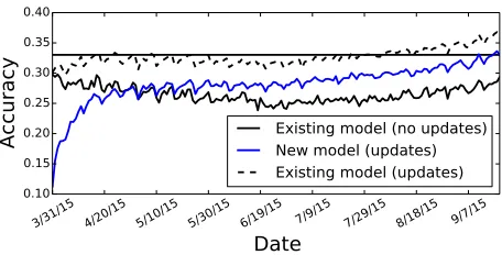
7 Question 3: Can periodic model updates maintain a trained geolocation system? Our results so far are sobering: shortly after a static model is deployed performance degrades to a model using two orders of magnitude less training data
(compare the drop in§6.2 with Figure 1). Increasing the amount of training data might be an option, but given our previous results on new users, etc., this is unlikely to be sufficient.
A simple method for addressing model degrada-tion over time is to continuously update the model over time using online learning on new data as it be-comes available. For example, we can continuously download a stream of (at least) 1% of geocoded tweets from the Twitter API to use as training for updating a deployed system. What is the impact on a system’s accuracy when it is updated on these geocoded tweets with SGD updates (§3)?
Figure 4 shows the performance of our system in an online setting (dashed black line). This model up-dates on every 100th example (1% of all geocoded tweets) encountered in the six-month evaluation pe-riod. When we update this previously trained static
3/31/15 4/20/15 5/10/15 5/30/15 6/19/15 7/9/15 7/29/15 8/18/15 9/7/15
Date
0.10 0.15 0.20 0.25 0.30 0.35 0.40
Accuracy
Existing model (no updates)New model (updates) [image:5.612.317.545.58.174.2]Existing model (updates)
Figure 4:Accuracy over the six months following train-ing. The horizontal line reflects the existing model’s per-formance on test from the same time period as training.
model, we see a quick recovery to accuracy levels that meet or exceed those on the test set from the same time period as training (horizontal line.)
Finally, we consider the case where a practitioner starts from scratch with no training data, but up-dates using just 1% of geocoded tweets. Can some-one with access to no prior training data build an effective model? Encouragingly, within 20 days the new model (solid blue line) catches the previ-ously trained static model (solid black line, “Ex-isting model: no updates“). This is an extremely promising result as it suggests that most practition-erswho do not have access to all geolocated data
can produce geolocation prediction models that ap-proximate models trained using hundred of millions of examples.
8 Conclusion
We have presented a tweet geolocation system that considers an order of magnitude more data than any prior work. Despite hundreds of millions of train-ing examples, the resulttrain-ing system is sensitive to the time the tweet was authored. Additionally, accuracy suffers when deployed on data beyond the training period. We show that online updates can mitigate problems caused by concept drift. In short, sheer volume of data is not enough: geolocation models should adapt to new data. Encouragingly, starting from no training data and updating on just 1% of geocoded tweets, within 20 days we can recover a model that catches a static model previously trained on hundreds of millions of tweets.
References
Alekh Agarwal, Olivier Chapelle, Miroslav Dud´ık, and John Langford. 2011. A reliable effective terascale linear learning system.CoRR, abs/1110.4198. David Broniatowski, Michael J. Paul, and Mark Dredze.
2013. National and local influenza surveillance through twitter: An analysis of the 2012-2013 in-fluenza epidemic. PLOS ONE, December 9.
Miriam Cha, Youngjune Gwon, and HT Kung. 2015. Twitter geolocation and regional classification via sparse coding. In Ninth International AAAI Confer-ence on Web and Social Media.
Ryan Compton, David Jurgens, and David Allen. 2014. Geotagging one hundred million twitter accounts with total variation minimization. InBig Data (Big Data), 2014 IEEE International Conference on, pages 393– 401. IEEE.
Mark Dredze, Michael J Paul, Shane Bergsma, and Hieu Tran. 2013. Carmen: A twitter geolocation system with applications to public health. InAAAI Workshop on Expanding the Boundaries of Health Informatics Using AI (HIAI).
John Duchi, Elad Hazan, and Yoram Singer. 2011. Adaptive subgradient methods for online learning and stochastic optimization. Journal of Machine Learning Research.
Jacob Eisenstein, Brendan O’Connor, Noah A Smith, and Eric P Xing. 2010. A latent variable model for ge-ographic lexical variation. In Empirical Methods in Natural Language Processing (EMNLP).
Kuzman Ganchev and Mark Dredze. 2008. Small sta-tistical models by random feature mixing. In Proceed-ings of the ACL08 HLT Workshop on Mobile Language Processing, pages 19–20.
Bo Han, Paul Cook, and Timothy Baldwin. 2014. Text-based twitter user geolocation prediction. Journal of Artificial Intelligence Research, pages 451–500. Liangjie Hong, Amr Ahmed, Siva Gurumurthy,
Alexan-der J Smola, and Kostas Tsioutsiouliklis. 2012. Dis-covering geographical topics in the twitter stream. In
Proceedings of the 21st international conference on World Wide Web, pages 769–778. ACM.
David Jurgens, Tyler Finethy, James McCorriston, Yi Tian Xu, and Derek Ruths. 2015. Geolocation prediction in twitter using social networks: A critical analysis and review of current practice. In Proceed-ings of the 9th International AAAI Conference on We-blogs and Social Media (ICWSM).
Juhi Kulshrestha, Farshad Kooti, Ashkan Nikravesh, and P Krishna Gummadi. 2012. Geographic dissection of the twitter network. InICWSM.
Brendan O’Connor, Michel Krieger, and David Ahn. 2010. Tweetmotif: Exploratory search and topic sum-marization for twitter. InInternational Conference on Weblogs and Social Media (ICWSM).
Miles Osborne, Sean Moran, Richard McCreadie, Alexander Von Lunen, Martin D Sykora, Elizabeth Cano, Neil Ireson, Craig Macdonald, Iadh Ounis, Yu-lan He, et al. 2014. Real-time detection, tracking, and monitoring of automatically discovered events in social media. InAssociation for Computational Lin-guistics (ACL).
Umashanthi Pavalanathan and Jacob Eisenstein. 2015. Confounds and consequences in geotagged twitter data. In Proceedings of the 2015 Conference on Empirical Methods in Natural Language Processing, pages 2138–2148, Lisbon, Portugal, September. Asso-ciation for Computational Linguistics.
Dominic Rout, Kalina Bontcheva, Daniel Preot¸iuc-Pietro, and Trevor Cohn. 2013. Where’s@ wally?: a classification approach to geolocating users based on their social ties. InProceedings of the 24th ACM Con-ference on Hypertext and Social Media, pages 11–20. ACM.