Proceedings of SemDeep-3, the 3rd Workshop on Semantic Deep Learning, pages 23–29 23
Automatically Linking Lexical Resources with Word Sense Embedding
Models
Luis Nieto-Pi ˜na University of Gothenburg [email protected]
Richard Johansson University of Gothenburg [email protected]
Abstract
Automatically learnt word sense embeddings are developed as an attempt to refine the capabilities of coarse word embeddings. The word sense representations obtained this way are, however, sensitive to underlying corpora and parameterizations, and they might be difficult to relate to word senses as formally defined by linguists. We propose to tackle this problem by devising a mechanism to establish links between word sense embeddings and lexical resources created by experts. We evaluate the applicability of these links in a task to retrieve instances of Swedish word senses not present in the lexicon.
1 Introduction
Word embeddings have boosted performance in many Natural Language Processing applications in re-cent years (Collobert et al., 2011; Socher et al., 2011). By providing an effective way of representing the meaning of words, embeddings facilitate computations in models and pipelines that need to analyze semantic aspects of language.
Based on their success, an effort has been concentrated in improving embedding models, from devising more computationally effective models to extending them to cover other semantic units beyond words, such as multi-word expressions (Yu and Dredze, 2015) or word senses (Neelakantan et al., 2014). Being able to represent word senses solves the problem of conflating several meanings of one polysemic word into a single embedding (Li and Jurafsky, 2015). Furthermore, having complete and accurate word sense representations brings embedding models closer to a range of existing, expert-curated resources such as lexica. Bridging the gap between these two worlds arguably opens a road to new methods that could benefit well-established, widely used resources (Faruqui et al., 2015; Speer et al., 2017).
This is the focus of the work we present in this article. We propose an automatic way of creating a mapping between entries in a lexicon and word sense representations learned from a corpus. By having an identification between a manual inventory of word senses and word sense embeddings, the lexicon obtains capabilities by which its entries can be manipulated as mathematical objects (vectors), while the vector space model receives support from a linguistic resource. Furthermore, by analyzing the disagree-ments between the lexicon and the embedding model, we can acquire insight into the shortcomings of their respective coverage. For instance, unlinked lexicon entries evidence those instances that the vector model is unable to learn, while unlinked word sense embeddings may suggest new usages of words found in the corpora. Being able to locate these cases opens the way towards improving lexica and embedding models. Automatic discovery of novel senses has been shown as a feasible and productive endeavor (Lau et al., 2012). In our evaluation we provide some insight into these situations: we use a mapping to calculate the probability that a word in a sentence from a corpus is an instance of an unlisted sense (i.e., not present in the lexicon.)
This mapping process, and some of its potential applications, are explained in detail in the following sections. Section 2 contains a description of the mapping mechanism Section 3 goes on to evaluate the performance of this mapping on finding instances of unlisted senses. We present our conclusions in Section 4.
2 Model
2.1 Lexicon
A lexicon which lists word senses and provides relations between them is required; for instance, a re-source that encodes these relations in a graph architecture, such as WordNet (Fellbaum, 1998).
We need to retrieve word senses related to any given target word sense in order to obtain a set of
neighbors which put the target sense in context. This context will be used to compare it with sets of neighbors extracted from a word sense vector space for senses of the same lemma, and thus find the best match to establish a link.
In our experiments on Swedish data we use SALDO (Borin et al., 2013) as our lexicon. It is encoded as a network: nodes encode word senses, which are connected by edges defined by semanticdescriptors: the meaning of a sense is defined by one or more senses, its descriptors. Among others, each sense has one primary descriptor(PD) and, in turn, it may be the primary descriptor of one or more senses. E.g., the PD of the musical sense of rockwould be music, which would be the PD ofhard rock. The PD network of SALDO traces back to aroot node(which does not have a PD) and, thus, it has a tree topology. In general, senses with more abstract meanings are closer to the root, while more concrete ones are located closer to the leaves.
2.2 Word Sense Embeddings
Word sense embeddings allow us to create an analogy between semantic relatedness among words and geometric distance between their representations in a vector space. In particular, a word sense embedding model assigns multiple representations to any given word, each of which is related to a distinct word sense. For our purposes, we make use of Adaptive Skip-gram (Bartunov et al., 2016), an adaptation of the hierarchical softmax Skip-gram (Mikolov et al., 2013).
The hierarchical softmax model is described by its training objective: to maximize the probability of context wordsvgiven a target wordwand the model’s parametersθ:
p(v|w, θ) = Y
n∈path(v)
1 1−e−ch(n)x>
wyn, (1)
wherexw are the input representations of the target wordsw, and the original output representations of
context wordsynare associated with nodes in a binary tree which has all possible vocabulary wordsvas
leaves;θis the set of these representations as weights of the vector model. In this context, path(v)are the nodesnin the path from the tree’s root to the leafv, identified by ch(n)being -1 or 1 depending on whethernis a right or left child.
The Adaptive Skip-gram (AdaGram) model expands this objective to account for multiple word senses to be represented in the input vocabularyX. It does so by introducing a latent variablezthat determines a concrete sensekof wordw. The output vocabularyY remains unchanged. This model uses a Dirichlet process (stick-breaking representation) to automatically determine the number of senses per word. They define a prior over the multiple senses of a word as follows:
p(z=k|w,β) =βwk k−1 Y
r=1
(1−βwr),
p(βwk|α) =Beta(βwk|1, α),
whereβis a set of samplesβ from the Beta distribution andαis a hyperparameter. By combining this prior with a pre-specified maximum number of prototypes and a threshold probability, the model is able to automatically determine the number of word senses any given word is expected to have. The objective function that defines the AdaGram model is defined as follows:
p(Y, Z,β|X, α, θ) =
V
Y
w=1
∞
Y
k=1
p(βwk|α) N
Y
i=1
p(zi|xi,β) C
Y
j=1
p(yij|zi, xi, θ)
Lexicon Vector space
rock-1‘jacket’ rock-b(clothing)
rock-2‘rock music’ rock-a,rock-c,
rock-d,rock-e(music)
Table 1: Example mapping forrock.
whereV is the word vocabulary size, N is the size of the training corpus,C is the size of the context window, and p(βwk|α) is the prior over multiple senses obtained via the Dirichlet process described
above. The granularity in the distinction between word senses is controlled by α. A trained model produces representations for word senses in a D-dimensional vector space where those with similar meanings are closer together than those with dissimilar ones.
For the purposes of this work, we trained a word sense embedding model on a Swedish corpus (cf. Section 3.1) using the default parameterization of AdaGram: 100-dimension vectors, maximum 5 pro-totypes per word, α = 0.1, and one training epoch. (See AdaGram’s documentation for a complete list.)
2.3 Lexicon-Embedding mapping
Our goal is to establish a mapping between lexicographic word senses and embeddings that represent the same meanings. The approach we take is to generate a set of related word senses for each sense of any given word, both from the lexicon (via relations encoded in its graph’s edges) and from the vector space (via cosine distance), to measure their relatedness and define mappings.
To obtain sets of neighbors from the lexicon, given any target word sense, any senses directly con-nected by an edge to the target’s node is selected as a neighbor. In the vector space, nearest neighbors based on cosine distance are selected.
In order to measure relatedness using geometric operations we need to assignprovisionalembeddings to lexicographic neighbors in order to measure their distance to vector space neighbors. We do this by using AdaGram’s disambiguation tool: given a target word and a set of context words, it calculates the posterior probability of each sense of the target word given the context words according to the hierarchi-cal softmax model (Equation 1). The word in context is disambiguated by selecting the its sense with the highest posterior probability. (In our case, for any given sense, the rest of senses in the set act as context.) We expect some lexicon-defined senses to not be present in the vector space and some word senses captured by the embedding model to not be listed in the lexicon. Additionally, the AdaGram model may create two or more senses for one word which relate to the same lexicographic sense. We address this by making the mapping 1-to-N to allow a lexicon sense to be linked to more than one sense embedding if necessary. Additionally, in order to make it possible for lexicon senses to be left unlinked, we propose to use afalse sense embeddingthat acts as an attractor for those lexicon senses with weak links to real embeddings.
The mapping mechanism is shown in Algorithm 1. For each word in the vocabulary, a set of neighbors is generated for each of its senses in the lexicon and in the vector space. The vector representations of these neighbors are averaged, since averaging embeddings has been proven an efficient approach to representing multi-word semantic units (Mikolov et al., 2013; Kenter et al., 2016). A probability matrix p ∈ [0,1]n×m is calculated by applying the softmax function to pairs of vectors. An extra column is added with scores generated by the softmax on zero-valued vectors to account for the false sense. A row inprepresents the probability that each sense in the vector model corresponds to that row’s lexicon sense, from which the maximum is obtained to establish a link. (A thresholdρexists to avoid low-probability links.)
Algorithm 1Mapping algorithm.
1: for allwordswdo
2: /* Lexicon neighbors */
3: n←#lexical senses ofw
4: si←ith lexical sense ofw,i∈[1, n] 5: for allsido
6: ai←set of neighbors ofsi 7: for allneighborkinaido
8: v(aik)←embedding foraik
9: end for
10: end for
11: /* Vector space neighbors */
12: T ←max #senses per word
13: m←#nearest neighbors (NN) per sense
14: zj←jth sense embedding ofw,j ∈[1, T] 15: for allzj do
16: bjl←lth NN ofbj,l∈[1, m]
17: end for
18: /* Average neighbors */
19: for alli,jdo
20: v(ai)←avg. vector overk
21: end for
22: for alljdo
23: v(bj)←avg. vector overl
24: end for
25: /* Mapping probabilities */
26: for alli,jdo
27: pij ←softmax(v(ai)·v(bj))
28: piN+1←softmax(
− →
0)
29: end for
30: /* Mapping */
31: forj∈[1, T]do
32: ifprior(sj)> ρthen
33: r←indmaxi(pij)
34: ifr 6=N + 1then
35: mapsrtozj
36: end if
37: end if
38: end for
39: end for
clothing-related meaning is linked to the sense meaning ‘jacket’, while the four music-related ones is linked to the sense meaning ‘rock music’.
3 Evaluation
3.1 Training Corpus
For training the AdaGram model, we created a mixed-genre corpus of approximately 1 billion words of contemporary Swedish downloaded from Spr˚akbanken, the Swedish language bank.1The texts were pro-cessed using a standard preprocessing chain including tokenization, part-of-speech-tagging and lemma-tization. Compounds were segmented automatically and when the lemma of a compound word was not listed in SALDO, we used the lemmas of the compound parts instead. For instance,golfboll‘golf ball’ would occur as a single lemma in the corpus, whilepingisboll‘ping-pong ball’ would be split into two separate lemmas.
3.2 Benchmark Dataset
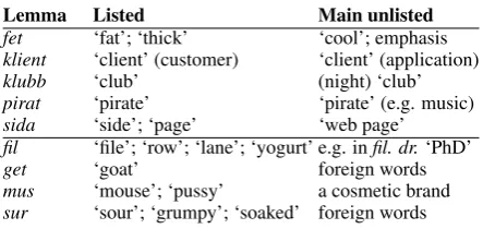
For evaluation, we annotated a benchmark dataset. We selected five target lemmas for which we knew that the corpus contains occurrences of word senses that are unlisted in the lexicon. In addition, we selected four target lemmas that do not strictly have new word senses, but that tend to be confused with tokenization artifacts, named entities, or foreign words. Table 2 shows the selected lemma, an overview of the senses that are listed in the lexicon, as well as the most important unlisted senses.
For each of these nine target lemmas, we selected 1,000 occurrences randomly from the corpus. Two annotators went through the selected occurrences and determined which of them are instances of the senses present in the lexicon, and which of them are unlisted senses. A small number of occurrences were discarded because they were difficult for the annotators to understand.
Lemma Listed Main unlisted
fet ‘fat’; ‘thick’ ‘cool’; emphasis
klient ‘client’ (customer) ‘client’ (application)
klubb ‘club’ (night) ‘club’
pirat ‘pirate’ ‘pirate’ (e.g. music)
sida ‘side’; ‘page’ ‘web page’
fil ‘file’; ‘row’; ‘lane’; ‘yogurt’ e.g. infil. dr.‘PhD’
get ‘goat’ foreign words
mus ‘mouse’; ‘pussy’ a cosmetic brand
[image:5.595.188.410.60.165.2]sur ‘sour’; ‘grumpy’; ‘soaked’ foreign words
Table 2: Selected target lemmas.
3.3 Experimental Settings
Given a mapping between lexicographic word senses and automatically discovered senses in a corpus, sentences from the benchmark dataset can be scored by their probability of containing an out-of-lexicon instance. A score is calculated using the linking probability between lexicographic senseyj and vector
model sensexi, P(yj|xi), and the probability of the AdaGram sensexi in the context of the sentence
ctx,P(xi|ctx):
P(yj|ctx) = T
X
i=1
P(yj|xi)P(xi|ctx),
thus obtaining the probability of a particular lexicographic senseyj given contextctx. The sum of all
p(yj|ctx),j ∈[1, T], yields the probability that an instance contains one of the listed word senses. Our
score, then, is calculated as the inverse probability:
score= 1−
n
X
j=1
P(yj|ctx). (3)
The human annotations of the sentences are interpreted as the gold standard, and the scores as our model’s classification output that can be used to rank the sentences from most to least probably containing an out-of-lexicon instance of a target word. We evaluate this classification using the Area Under the Receiver Operating Characteristic Curve (AUC). For reference, recall that the expected AUC of a random ranking is 0.5.
The potential of the automated mapping between a lexicon and an embedding model to help retrieve instances of word senses unlisted in the lexicon gives us a certain measure of the quality of this mapping. The recovery of instances of unlisted senses can only succeed if the mapping has successfully identi-fied listed lexicon senses in the embedding model, leaving unlisted ones unlinked. On the other hand, failure to recover instances of unlisted senses can expose weaknesses in the automated mapping. (See Section 3.4 for an analysis of unsuccessful cases.)
3.4 Results
We apply the scoring and evaluation process explained above on the sets of sentences for each of the words selected for the benchmark dataset. Table 3 summarizes the results obtained. We observe a clear
Word n AUC
fet 976 0.76
klient 959 0.02
klubb 985 0.74
pirat 907 0.53
sida 985 0.69
Sub-avg. 0.55
(a) Unlisted senses.
Word n AUC
fil 982 0.87
get 954 0.98
mus 972 0.83
sur 967 0.96
Sub-avg. 0.91 Total avg. 0.73
(b) Spurious senses.
difference between the two types of lemmas: the model’s performance is notably higher when the lemmas may be confused with tokenization artifacts, named entities or foreign words (Table 3b) than when the lemmas have meanings not listed in the lexicon (Table 3a). This is arguably due to the ability of the word sense embedding model to isolate spurious meanings in the vector space since these occurrences tend to be distributionally quite distinct from the standard uses. However, note that also for the case of unlisted meanings, the model generally improves over a random baseline.
The exception to this is the case of klient, where the listed sense is ‘customer’ and the new sense is ‘client application’. Here, the ranking is upside down, as can be seen from the very low AUC value. The cause of this issue can be traced to the inability of the mapping algorithm to successfully link the only lexicographic sense to its corresponding vector space embedding. The neighbors of the AdaGram sense corresponding to the ‘customer’ sense tend to be legal terms, which are not connected to this sense in the lexicon. (Arguably, the legal use of ‘client’ could be seen as a separate sense.) Compare this to the case ofpirat, which performs roughly at random (AUC≈0.5), suggesting simply that the AdaGram model has not picked up the distinction between the senses, which makes it hard to solve the problem by simply changing the link, as would be the case withklient.
A straightforward way to address those cases in which the mapping fails to correctly establish a link would be to refine the way in which the word senses are represented at the time of linking. Our approach is to do this by averaging the embeddings of nearest neighbors, due to the simplicity and usual robustness of this operation. However, more complex approaches to combining embeddings have been demonstrated using, for example, weighted averaging (Arora et al., 2017), which could be adapted for our needs in this work.
4 Conclusion
We have presented an approach to automatically link lexicographic word senses with word sense em-beddings by retrieving sets of senses related to the different meanings of a lemma and measuring the similarity between their vector representations. We argue that potential applications of such a system resides on those embeddings that cannot be linked to a lexicographic sense, as this could serve to sug-gest potential new entries to the lexicon, or to filter unlisted instances from a corpus. To illustrate this point, the evaluation of our system has been focused on its ability to retrieve instances assumed to belong to unlisted senses. Our system is able to identify such instances in many cases, as its performance in terms of AUC is above that of a random baseline. The performance is specially high in cases where the target lemma can be confused in the corpus with spurious meanings such as foreign words. In sum-mary, our results indicate that establishing links between existing resources and embedding models has potential applications in NLP tasks which require formal lexicographic knowledge. In the future, we propose to examine ways to improve the current mapping system with improved neighbor representation approaches, as well as to investigate further possible uses, such as improving existing resources with data obtained from corpora.
Acknowledgements
This research was funded by the Swedish Research Council under grant 2013–4944.
References
Sanjeev Arora, Yingyu Liang, and Tengyu Ma. 2017. A simple but tough-to-beat baseline for sentence embed-dings. InInternational Conference on Learning Representations (ICLR).
Sergey Bartunov, Dmitry Kondrashkin, Anton Osokin, and Dmitry P. Vetrov. 2016. Breaking sticks and ambigui-ties with adaptive skip-gram. InProceedings of the 19th International Conference on Artificial Intelligence and Statistics (AISTATS).
Lars Borin, Markus Forsberg, and Lennart L¨onngren. 2013. SALDO: a touch of yin to WordNet’s yang. Language
Ronan Collobert, Jason Weston, L´eon Bottou, Michael Karlen, Koray Kavukcuoglu, and Pavel Kuksa. 2011. Natural language processing (almost) from scratch.The Journal of Machine Learning Research, 12:2493–2537.
Manaal Faruqui, Jesse Dodge, Sujay Kumar Jauhar, Chris Dyer, Eduard Hovy, and Noah A Smith. 2015. Retrofitting word vectors to semantic lexicons. InProceedings of the 2015 Conference of the North American
Chapter of the Association for Computational Linguistics: Human Language Technologies, pages 1606–1615.
Christiane Fellbaum, editor. 1998.WordNet: An electronic lexical database. MIT Press.
Tom Kenter, Alexey Borisov, and Maarten de Rijke. 2016. Siamese cbow: Optimizing word embeddings for sentence representations. In Proceedings of the 54th Annual Meeting of the Association for Computational
Linguistics (Volume 1: Long Papers), volume 1, pages 941–951.
Jey Han Lau, Paul Cook, Diana McCarthy, David Newman, and Timothy Baldwin. 2012. Word sense induction for novel sense detection. InProceedings of the 13th Conference of the European Chapter of the Association for Computational Linguistics, pages 591–601. Association for Computational Linguistics.
Jiwei Li and Dan Jurafsky. 2015. Do multi-sense embeddings improve natural language understanding? In
Proceedings of the 2015 Conference on Empirical Methods in Natural Language Processing, pages 1722–1732.
Tomas Mikolov, Ilya Sutskever, Kai Chen, Greg S Corrado, and Jeff Dean. 2013. Distributed representations of words and phrases and their compositionality. InAdvances in Neural Information Processing Systems, pages 3111–3119.
Arvind Neelakantan, Jeevan Shankar, Alexandre Passos, and Andrew McCallum. 2014. Efficient non-parametric estimation of multiple embeddings per word in vector space. InProceedings of the 2014 Conference on
Empir-ical Methods in Natural Language Processing (EMNLP), pages 1059–1069, Doha, Qatar, October. Association
for Computational Linguistics.
Richard Socher, Eric H Huang, Jeffrey Pennin, Christopher D Manning, and Andrew Y Ng. 2011. Dynamic pooling and unfolding recursive autoencoders for paraphrase detection. InAdvances in Neural Information
Processing Systems, pages 801–809.
Robert Speer, Joshua Chin, and Catherine Havasi. 2017. Conceptnet 5.5: An open multilingual graph of general knowledge. InAAAI, pages 4444–4451.