Journal of Experimental Psychology:
Animal Learning and Cognition
Ratios and Effect Size
Jasper Robinson
Online First Publication, August 14, 2017. http://dx.doi.org/10.1037/xan0000143
CITATION
Robinson, J. (2017, August 14). Ratios and Effect Size. Journal of Experimental Psychology:
Animal Learning and Cognition. Advance online publication.
Ratios and Effect Size
Jasper Robinson
University of Nottingham
Responding to a related pair of measurements is often expressed as a single discrimination ratio. Authors have used various discrimination ratios; yet, little information exists to guide their choice. A second use of ratios is to correct for the influence of a nuisance variable on the measurement of interest. I examine 4 discrimination ratios using simulated data sets. Three ratios, of the forma/(a⫹b),b/(a⫹b), and (a⫺b)/(a⫹b), introduced distortions to their raw data. The fourth ratio, (b⫺a)/blargely avoided such distortions and was the most sensitive at detecting statistical differences. Effect size statistics were also often improved with a correction ratio. Gustatory sensory preconditioning experiments involved mea-surement of rats’ sucrose and saline consumption; these flavors served as either a target flavor or a control flavor and were counterbalanced across rats. However, sensory preconditioning was often masked by a bias for sucrose over saline. Sucrose and saline consumption scores were multiplied by the ratio of the overall consumption to the consumption of that flavor alone, which corrected the bias. The general utility of discrimination and correction ratios for data treatment is discussed.
Keywords:effect size, discrimination learning, discrimination ratio, suppression ratio, reduction
Supplemental materials:http://dx.doi.org/10.1037/xan0000143.supp
I examine the use of two methods for treating data to maximize statistical sensitivity: transforming dataintoa discrimination ratio, and treating datawitha ratio that corrects for the influence of an unwanted variable. It is generally useful to apply a transformation to data (e.g., Howell, 2002). This may be to better meet assump-tions for parametric analysis (e.g., log transformation of negatively skewed latency data; see, e.g., Miller, Laborda, Polack, & Miguez, 2015). A different motive is to improve statistical sensitivity. Discrimination ratios (e.g.,a/(a⫹b), Kamin, 1969), see below for full description) offer two important benefits: In addition to sim-plifying analysis by converting a pair of raw numbers (e.g., in-strumental response rates during conditioned stimulus and baseline measurements) into a single ratio, the discrimination ratio can reduce subject-by-subject variability because of its accommoda-tion of baseline (b) response rates. It is this second feature of the
discrimination ratio that offers improved statistical sensitivity. Rather little is known about discrimination ratios’ properties. To this end, I describe analyses that use synthetic data to characterize the effects of discrimination ratios on data and especially on their statistical sensitivity. In the second section of this report I describe empirical data whose effect of interest is masked by the influence of the specific stimuli used. In these sensory preconditioning experiments, rats’ preference for a control flavor over one with aversive properties was, in many experiments, masked by an overriding preference for sucrose over saline. Sucrose and saline were counterbalanced to serve as either the control or the aversive flavor. I describe a simple method for correcting for the intrinsic sucrose-saline bias seen in such experiments and examine its effects on statistical sensitivity.
Data Treatment
For analyses of both discrimination ratios and the correction ratio, standard parametric analyses were used for null-hypothesis testing. Tests evaluated two-tailed hypotheses and ␣ ⫽ .050. Partial eta squared (p2) was used to represent main effect and interaction effect sizes. Standardized 90% confidence intervals (CIs) forp2were computed using the methods described by Kelley (2007) and used his MBESS package for R (Version 3.3.2. [Com-puter software], Vienna, Austria). Bayesian analyses supplemented the interpretation of a key results (JASP (Version 0.8 Beta 5) [Computer software]. Amsterdam, The Netherlands). The Bayes factor (BF) specifies the ratio of the probabilities between a target model (BF10) and an appropriate comparison, such as the null model (BF01). The magnitude of the ratio is taken to reflect the likelihood of the support for the target model, which may be instructive in interpreting data. Jeffreys (1961, as cited in, Rouder, Speckman, Sun, Morey, & Iverson, 2009) maintained that BFs greater than 3 may be considered “some evidence” for one
hy-Work reported here was funded by the Biotechnology and Biological Sciences Research Council to JR (BB/C006283/1). Procedures were au-thorized under United Kingdom law, Animals (Scientific Procedures) Act (1986; PCD40/2406, PPL40/2868, PIL30/6232). I am grateful to Pete Bibby and Charlotte Bonardi for their helpful discussion, to Pia Robinson for comments on a draft of this report and to Dave George for sharing his code for creating surface plots.
This article has been published under the terms of the Creative Com-mons Attribution License (http://creativecomCom-mons.org/licenses/by/3.0/), which permits unrestricted use, distribution, and reproduction in any me-dium, provided the original author and source are credited. Copyright for this article is retained by the author(s). Author(s) grant(s) the American Psychological Association the exclusive right to publish the article and identify itself as the original publisher.
Correspondence concerning this article should be addressed to Jasper Robinson, School of Psychology, University of Nottingham, United Kingdom.
pothesis over its alternative hypothesis, with BFs of 10 or more or 30 or more as, respectively, “strong” and “very strong” evidence.
Four Discrimination Ratios
Kamin (1969) used the discrimination ratio, a/(a ⫹ b), in conditioned suppression experiments. Whenais nonnegative and
bis greater than zero, the ratio will vary between 0 and 1.0 with 0.5 corresponding to a and bhaving equivalent values. In a condi-tioned suppression experiment, arepresents the instrumental re-sponse rate (e.g., Bonardi & Jennings, 2009; Robinson, Whitt, Horsley, & Jones, 2010) or lick rate (e.g., Pezze, Marshall, & Cassaday, 2016) during a conditioned stimulus for shock (condi-tional stimulus [CS] rate); andbrepresents a baseline response rate (e.g., the instrumental or lick rate immediately before the presen-tation of the conditioned stimulus; Pre-CS rate). Here, similar CS and Pre-CS rates will yield ratios that approximate 0.5. They will approach zero as responding to the conditioned stimulus becomes suppressed, for example during the acquisition of the conditioned response. Another purpose is to simplify the performance of birds in an appetitive discrimination (e.g., George & Pearce, 1999). Here
aand bmight be the response rates of, respectively, food rein-forced and nonreinrein-forced stimuli. Successful discrimination is reflected ina’s values exceedingb’s and in discrimination ratios rising from chance (0.5) to approach 1.0 (see also, Harris, Shand, Carroll, & Westbrook, 2004; Montuori & Honey, 2016).
Other ratios are possible that capture the discrimination between a pair ofaandbvalues and I will describe three that have been used in experimental psychology. Redhead has reported data from an appetitive discrimination with pigeons in whichaandbrefer, respectively, food-reinforced and nonreinforced conditioned stim-uli (Redhead & Curtis, 2013; Redhead & Pearce, 1998). They used the ratiob/(a⫹b) to capture each bird’s discrimination. Birds’
performance began at around 0.5 and progressed toward 0 as responding became focused on the food-reinforced trials, repre-sented bya. A third ratio was used by Ennaceur and Delacour (1988) to summarize discrimination of rats’ exploration of novel (a) and familiar (b) junk objects in recognition memory experi-ments. Their ratio has the form (a⫺b)/(a⫹b). Rats’ biased their exploration toward the novel object, represented by a, giving positive Ennaceur ratios (i.e., 1ⱖratio⬎0). Notice that the three ratios’ share their denominator but differ in their numerator. The fourth ratio that I will consider has a different denominator and the form: (b ⫺ a)/b. This ratio was used by Pfautz, Donegan, and Wagner (1978; see also Hoffman, Selekman, & Fleshler, 1966) in Pavlovian shock conditioning experiments with rats and rabbits.a
andbrefer, respectively, to the response rates (lever pressing or heart rate) during the conditioned stimulus and to the baseline rate. Pfautz ratios are zero when a is equivalent to b (e.g., before conditioning has taken place) and approach one as responding is suppressed during the conditioned stimulus. All four of these ratios have the advantage over a simple ratio (e.g.,a/b) that they will be bound within a fixed range of values. The properties of these four ratios were characterized by systematically generating data sets and comparing them to one another. These simulations were in-tended to help to understand potential distortions that each ratio produces from the primary data and to assess potential differences in their statistical sensitivity.
Surface Plots of the Four Discrimination Ratios
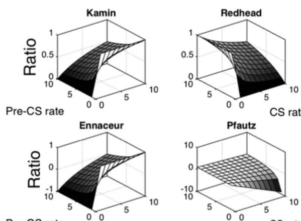
[image:3.603.145.445.464.685.2]The top left surface plot of Figure 1 displays the relationship betweena(e.g., CS) andb(Pre-CS) rates and Kamin ratios using hypothetical data. The Matlab code and figure are included in the supplemental materials. The Matlab figure allows rotation of the surface plots and specification of the axis values to facilitate
inspection. The ordinate indicates the Kamin ratios that are derived when Pre-CS and CS rates are each varied between 0 and 10 in one-step intervals. The rear left panel of the surface plot indicates data derived when CS rates do not exceed Pre-CS rates, as in a conditioned suppression experiment (e.g., Bonardi & Jennings, 2009; Robinson et al., 2010); the rear right panel of the surface plot indicates data derived whenarates do exceedbrates (cf., George & Pearce, 1999). Kamin ratios will approach 0 as CS rates ap-proach zero and 1.0 as Pre-CS rates apap-proach 0. Despite the one-step intervals between each CS and Pre-CS response rate being linear, their relationship to the Kamin ratio is nonlinear. In particular, the relationship bows as the Pre-CS and CS rates reach parity (i.e., where the Kamin ratio equals⫽0.5).
The top right, and lower pair of surface plots in Figure 1 demonstrate the relationship between a and b rates using, the Redhead (Redhead & Curtis, 2013; Redhead & Pearce, 1998), Ennaceur (e.g., Ennaceur & Delacour, 1988), and Pfautz (Pfautz et al., 1978) ratios. The Ennaceur ratio produces an identically shaped plot to the Kamin ratio, albeit with a different range of ratio values. The Redhead ratio produces a plot having the mirror image of the Kamin ratio plot and has the same range of values. The Ennaceur ratio will yield ratios approaching minus one in condi-tioned suppression experiment where Pre-CS ratios (b) exceed CS ratio (a; e.g., Robinson, Sanderson, Aggleton, & Jenkins, 2009). At parity the rates will give a ratio of zero and when thearate exceeds the b rate Ennaceur ratios approach positive one (e.g., Ennaceur & Delacour, 1988; Whitt, Haselgrove, & Robinson, 2012; Whitt & Robinson, 2013). The Redhead ratio will be zero withaandbrate parity and will mirror the Kamin ratio both in typical conditioned suppression ratio experiments (i.e., ratios ap-proach one rather than zero during suppression) and in appetitive discrimination experiments (i.e., ratios approach zero rather than one on master of the discrimination; e.g., Redhead & Curtis, 2013; Redhead & Pearce, 1998). The Pfautz ratio’s surface plot is dif-ferent from those of the other three ratios. Although the ratio’s surface plot becomes nonlinear when Pre-CS rates are low and CS rates are high (i.e., the bottom right region of the surface plot’s box), elsewhere it retains much more of the linearity of the CS and Pre-CS rates (note that this linearity is more evidence in Figure 3, which is discussed below).
Comparison of Effect Sizes From Kamin
and Pfautz Ratios
The previous examination of the Kamin, Ennaceur, and Red-head ratios indicated that, although the specific values of the ratios differed, they behaved similarly in their representation of CS and Pre-CS rates. In particular, the ratios’ surface plots and the effect sizes of their one-sample-tstatistics were similar. Because of that similarity, the current analysis considers only one of those three (the Kamin ratio), and compares it to the Pfautz ratio, whose characteristics are different.
Simulations methods. R (Version 3.3.2. [Computer
soft-ware], Vienna, Austria) was used to generate 500 normally dis-tributed data points that varied around a mean of 1 and had aSD
of 0.1. These were to serve as theavalues in a population of 500 Kamin ratios. The code is included in the supplemental materials. Theadistribution generation was initiated using the “seed” num-ber 1. Simulations using the same seed produced the same
distri-bution, allowing identical simulations to be created when needed. A second and third distribution was created using the same process and the same seed number but theSDs were increased to 0.2 and to 0.3. The process for the generation of a trio ofadistributions with means of 1 was repeated for distributions with means of 8, 15, 22, 29, 36, and 43; thus, being equally spaced and symmetrical with respect to the midpoint, 22. These steps created a series of 18
a-distributions with three different standard distributions, six dif-ferent means and the same seed value, 1. The process was repeated with new seeds taken from the natural integer series: 2, 3, 4. . . . To prevent the subsequent generation of unusual ratios (i.e., ⬎1 and⬍0), normal distributions that generated negative values were not used. Eight seeds were used in total and these processes yielded 144 sets of normally distributed data (i.e., eight seeds⫻ six means⫻3SDs).
The process for generation of Kamin ratios was repeated for the Pfautz ratios. The same seeds were used to permit meaningful comparison of the ratios that were generated.
Next all data were used to compute Kamin and Pfautz ratios with a fixedbvalue of 22, that is, the midpoint on theaseries. Except for ratios based on a distributions with a mean of 22, one-sample t, and associated, statistics were calculated for the ratios, with the Kamin ratios being compared with ⫽0.5 and the Pfautz ratio being compared with ⫽0.0. The statistics were used to examine possible variation in the level of sensitivity to detect differences fromacross the profile of ratios.
Simulation results. Two seeds in the natural integer se-quence, 1–10, yieldeda-distributions that were discarded because their seed created one or more negative values. This left eight
[image:4.603.335.517.545.654.2]a-distributions that contained no negative values. An example of Kamin-ratio data based on a-distributions having aSD of .3 is given in Figure 2. As the mean values increased across the series (i.e., 1, 8, 15, 22, 29, 36, and 43) the ratios increased, a pattern that may be likened to the extinction of conditioned suppression (e.g., Ward-Robinson & Hall, 1999). Notice that the Kamin ratios in-crease nonlinearly and cluster in the region where a becomes equivalent tob, just as Figure 1 depicts. Or, as an alternative view, the pairs of meanarates 1 and 43, 8 and 36, and 15 and 29 are equivalently distant from the brate, 22, but their ratios are not equidistant. A third feature is that the lower the mean value of the distribution, the greater the variability of the Kamin ratios. The
Figure 2 data correspond to the Kamin surface-plot in Figure 1. In particular, the Figure 2 data correspond to the ratios on the back surfaces of the surface plot (most of the left side and a smaller portion of the right side nearest the corner). The code for the generating the ratios is available in the supplemental materials.
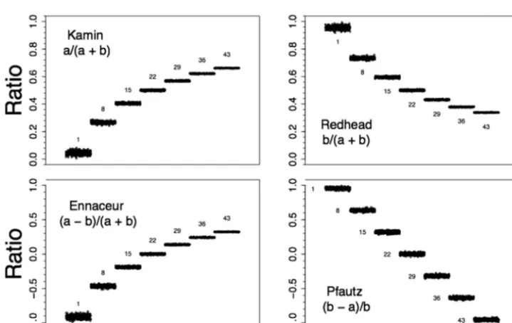
Example data from all four ratios are presented in Figure 3. Example code is given in the supplemental materials. The ratio data are from simulations with theSDof .3 and, from right to left, indicate ratios that might be found during extinction of conditioned suppression (e.g., Ward-Robinson & Hall, 1999). All data in Figure 3 were computed based on distributions having the same random seed number. The Ennaceur ratio produced a similar distribution of ratios as the Kamin ratio, albeit with values on a different scale; that is: (a) The lineara-rates produced nonlinear ratios; and (b) There was greater variability in ratios associated with lowera-rates. The Redhead and Pfautz ratio declined in value as theavalues increased. The Redhead ratio produced a similar nonlinear profile as the Kamin and Ennaceur ratios and, likewise, had greater variability in ratios associated with lowera-rates. As was seen in Figure 1, the Pfautz ratio differs from the other three ratios in that the linear sequence in thearates is retained in its ratios. Another difference is that the variability is similar across ratios computed from data with all levels ofarate. This description of the data was supported by linear-regression analysis: The Pfautz data in Figure 3 were perfectly described as linear trends,R2 ⫽ 1.000; the remaining three ratios’ data were more accurately de-scribed as cubic trends, 0.996ⱕR2ⱕ0.999, than linear, 0.910ⱕ
R2ⱕ0.990, or quadratic trends, 0.993ⱕR2ⱕ0.996.
Table 1 gives further information about the properties of the four types of ratio. Its upper panel simply gives the ratios for each of thearates (CS rate) with abrate (Pre-CS rate) of 22. The ratio thus approximates the simulated data in Figure 3.
Comparison is made of the seven ratios of each type to its value. Mu is taken as the ratio value where CS and Pre-CS rates are both 22. Comparison is made using one-samplettests and associatedpand effect sizes are given. The average of the seven ratios differs across the four ratios but the absolute difference
between the mean ratio and is the same for the Kamin and
Redhead ratios. The Kamin, Redhead, and Ennaceur ratios sharet,p, and effect size statistics. The Pfautz ratio stands alone in this comparison: With the rates used here, the ratios are more sensitive in that the one-sample t was better able to detect a difference from.
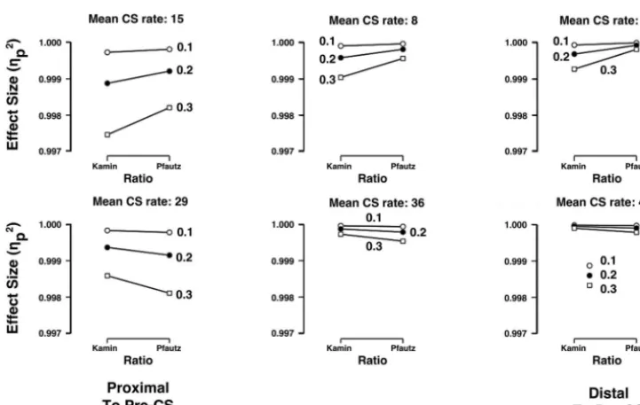
Analysis of effect sizes from kamin and pfautz ratios. The Kamin and Pfautz ratios that were generated above were eval-uated by reference to their respectives (i.e., 0.5 for the Kamin ratio and 0 for the Pfautz ratio) using one-samplettests whose effect size statistics are summarized in Figure 4. Raw data and statistical analysis are supplied in the supplemental materials. The simulated data had smallSDs and largens (n⫽500), which produced large effect sizes. The data show that effect sizes were, unsurprisingly, larger from ratios based on smallerSDs. Ratios that were based on CS rates that were proximal to the Pre-CS rate, 22, (i.e., from distributions with averagearates of 15 or 29) were lower than ratios based onarates further from 22, especially in combination with largerSDs. This is especially clear in the ratios whose CS rates averaged 1 and 43, with rates of 8 and 36 being in-between the two extremes. Most significant was the variation in the effect sizes of the Kamin and Pfautz ratios. The top row summarizes data that correspond to condi-tioned suppression, that is, where the mean CS rates (15, 8, and 1) are lower than the Pre-CS rate. Here, the Pfautz ratio ap-peared to produce superior effect sizes to the Kamin ratio. The reverse appeared to be the case in elevated ratios, those
[image:5.603.117.477.448.675.2]marized in the lower row with mean CS rates are higher than the Pre-CS rate, 22.
To simplify and focus the main features of the simulated ratio data, they were recoded with theSDvariable omitted and with the
[image:6.603.120.477.111.268.2]mean-CS-rate variable recoded more crudely as being suppressed or elevated (i.e., either above or below the Pre-CS rate of 22). These simplified data are summarized in Figure 5. The effect sizes from Kamin ratios were higher when they were based on elevated Table 1
One-Sample t-Statistics for Four Different Methods for Discrimination Ratio Computation With Varied CS (B) Rates and a Fixed Pre-CS (a) Rate
Kamin a/(a⫹b)
Redhead a/(a⫹b)
Ennaceur (a⫺b)/ (a⫹b)
Pfautz (b⫺a)/b
CS rate Ratio Ratio Ratio Ratio
[image:6.603.116.477.408.636.2]1 .0435 .5000 .9565 .5000 .9130 .0000 21.0000 .0000 8 .2667 .5000 .7333 .5000 .4667 .0000 1.7500 .0000 15 .4054 .5000 .5946 .5000 .1892 .0000 .4667 .0000 22 .5000 .5000 .5000 .5000 .0000 .0000 .0000 .0000 29 .5686 .5000 .4314 .5000 ⫺.1373 .0000 ⫺.2414 .0000 36 .6207 .5000 .3793 .5000 ⫺.2414 .0000 ⫺.3889 .0000 43 .6615 .5000 .3385 .5000 ⫺.3231 .0000 ⫺.4884 .0000 Effect size (p2)⫽ .0847 — .0847 — .0847 — .1569 — t(6)⫽ .7450 — .7450 — .7450 — 1.0565 — p⫽ .4844 — .4844 — .4844 — .3314 — Mean ratio⫽ .4381 — .5619 — .1239 — 3.1569 — |Mean ratio⫺ |⫽ .0619 — .0619 — .1239 — 3.1569 —
Note. CS⫽conditional stimulus. Four different discrimination ratios computed for seven CS rates with a fixed Pre-CS rate, 22. In the formula,aandb, respectively, refer to the CS and Pre-CS rates. The ratio value when the CS rate is equivalent to the Pre-CS rate () is presented to the right of each ratio. The lower portion of the table depicts the results of a one-samplet-test for each of the four types of ratio with the associated effect size and pstatistics. The mean of each set of ratios and the absolute difference between each mean andare presented below this.
CS rates than on suppressed CS rates. By contrast, the Pfautz ratios’ effect sizes appeared unaffected by their side of the Pre-CS. This description of the data was supported by ANOVA (analysis of variance), which did not detect a main effect of the Kamin versus Pfautz ratios,F(1, 284)⫽1.6;p⬎.196;p2⬍.007, 90% CI [.000, .029]. However, the ANOVA detected a main effect of suppression versus elevation,F(1, 284)⫽9.5;p⬍.003;p2⬎.031, 90% CI [.007, .072], and a Kamin/Pfautz⫻Suppression/Elevation inter-action, F(1, 284)⫽ 10.8; p⬍ .002; p2 ⬎ .036, 90% CI [.009, .078]. The source of this interaction was investigated with simple main effects analyses, using the common-error term. The effect size difference in elevated Kamin and Pfautz ratios was unreliable,
F(1, 284)⫽2.0;p⬎.161;p2⬍.006, 90% CI [.000, .031], but the corresponding difference for suppressed ratios was reliable,F(1, 284)⫽10.5;p⬍.002;p2⬎.035, 90% CI [.008, .076]. Elevated Kamin ratios were reliably higher than suppressed Kamin ratios,
F(1, 284)⫽20.3;p⬍.001;p2⬎.066, 90% CI [.026, .116], but no such elevation/suppression difference was detected for Pfautz ratios,F⬍1;p⬎.89;p2⬍.001, 90% CI [.000, .005]. A Bayesian ANOVA was performed with models corresponding to the previ-ous ANOVAs variables and matched its findings. The model based on the Kamin/Pfautz ⫻ Suppression/Elevation interaction was strongly favored over the combined Kamin/Pfautz and Suppres-sion/Elevation models, BF10⬎23.7. These analyses are included in the supplemental materials.
This analysis indicated that the Pfautz ratio behaved similarly to suppressed and to elevated CS rates: Effect size statistics associ-ated with one-samplets were indistinguishable by inferential test-ing. By contrast the Kamin ratio produced greater effect size
statistics with elevated data than with suppressed data. It is notable that the absolute differences in the effect sizes are trivially small and might lead one to conclude that all of the ratios produce excellent effect sizes. However, the synthetic data used here have large sample sizes and this will boost effect size statistics to points beyond those typically seen in empirically obtained data. Further-more, because p2 will not exceed 1 the absolute differences in these synthetic data are likely to be compressed. Thus, the absolute difference in the effect size statistics in empirical data is likely to be greater than that seen here.
Discussion
The Kamin (1969), Redhead (Redhead & Curtis, 2013; Redhead & Pearce, 1998), and Ennaceur (e.g., Ennaceur & Delacour, 1988) ratios produced similar distortions on the simulated conditioned suppression data. Ratios based on low CS rate (a) had greater variability than CS rates that were similar to the Pre-CS rate (b). Furthermore, the space between the ratios corresponding to neigh-boring CS rates was uneven: Rather than corresponding to the equal steps between each CS rate, they were relatively compressed as the CS rate approximated the Pre-CS rate. The Pfautz ratio (Pfautz et al., 1978) suffered neither of those complications: Ratios for different CS rates did not differ in their variability and the interval between each set of ratios retained the linearity of the original CS rates.
The Kamin and Pfautz ratios differed in their sensitivity as measured by effect size statistics based on one-samplettests that compared each CS-rate’s population of ratios to the value of the ratio when theaandbrates were equal. In particular, the Kamin ratio suffered a marked loss in effect size when thea-rate was far lower than the b-rate, the situation in conditioned suppression experiments. The implication of this is that we should not use Kamin’s ratio for conditioned suppression experiments, or any other procedure in which the aim is to detect effects whena⬍b. Instead, we should favor Pfautz’ ratio. The Kamin ratio has been favored in conditioned suppression experiments for the last five decades and these new findings indicate that effect sizes may have been underestimated.
The Kamin ratio produced better effect sizes when the CS rate (a) exceeded the Pre-CS rate (b). This arrangement is often seen in experiments where thea-rate rises during mastery of a discrimi-nation and theb-rate may either decline or remain an estimate of a constant baseline rate (e.g., George & Pearce, 1999; Harris et al., 2004; Montuori & Honey, 2016). The implication of these simu-lations is that the Kamin ratio is a suitably sensitive treatment for such data. Although there was no inferential statistical support for the observation, the mean value for the Kamin ratio whena⬎b
was the largest of the four ratios. The Pfautz ratio’s effect sizes were indistinguishable when applied to data of either form (i.e.,
either a ⬍ b or a ⬎ b). The natural conclusion from these
observations is that the Pfautz ratio should be used by default: It does not distort its input data and produces robust effect sizes that are equal for botha⬍bora⬎bdata.
I emphasize that these conclusions are based on very large sets of synthetic data that may detect ratio differences in effect size that would be rendered marginal in real experimental data with smaller
ns. Nevertheless, researchers are encouraged to report effect sizes, not only for their own individual experiment, but to allow
gated effect sizes to be computed that are based onmanysimilar experiments (e.g., Cumming, 2011; Lakens, 2013). Thus, even small differences in the effect sizes from particular ratios may ultimately become important.
Skewed data sets could benefit from the distorting influence of some of these ratios. Consider lick-suppression, latency data (e.g., Miller et al., 2015; Pezze et al., 2016) that will often be negatively skewed: They will be relatively diffuse at long latencies and compressed at short latencies, as they approach the floor of zero seconds. This pattern of compression and expansion is the com-plement of the distortions appreciable in Figure 3 seen for the Kamin, Redhead, and Ennaceur ratios. Thus, depending upon the level of responding at which key effects are to be detected, these ratios could outperform the Pfautz ratio with negatively skewed data.
A Correction Ratio to Eliminate the Influence of a
Nuisance Variable on Effect Size
The motive for applying the discrimination ratios above is to reduce data variability to better support statistical analysis. The discrimination ratios achieve this by compensating for subject-by-subject variation in one variable (e.g., Pre-CS rate) to allow more sensitive data analysis of the target variable (e.g., CS rate). I now describe a second ratio-based technique to reduce variance to improve data sensitivity. Rather than operate at subject-by-subject variability, this method applies a correction ratio to offset distor-tions produced by nuisance variables. I exemplify this with an example from a gustatory sensory preconditioning procedure in which the nuisance variable is based on intrinsic differences in rats’ consumption of two flavored solutions. This interferes with detection of differences in consumption based on the experimental treatment. The correction ratio technique is quite general and broader applications will be considered.
An Application of the Correction Ratio to
Sensory Preconditioning
Rescorla and Cunningham (1978) reported within-subject sen-sory preconditioning data with rats. Their procedure involved rats first receiving a pair of compound flavors on separate trials (e.g., sucrose-acid and saline-quinine). To reveal learning about the co-occurrence of each pair of flavors, one flavor (e.g., acid) was paired with illness to create an aversion to it. Rescorla and Cun-ningham reported a marked reduction in consumption of the flavor whose partner was illness-paired (i.e., sucrose in this example). The experiment was counterbalanced such that for half of the rats, sucrose was made aversive and saline was the control flavor and for the remaining rats saline was aversive and sucrose was the control flavor. Although successful in demonstrating sensory pre-conditioning, there was a pronounced overall preference for su-crose over saline during testing. This preference may have acted against Rescorla and Cunningham detecting sensory precondition-ing (see also Ward-Robinson, Symonds, & Hall, 1998).
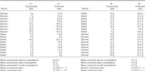
Unpublished data from a similar sensory preconditioning pro-cedure are presented in Table 2. Uncorrected fluid consumption data, measured in grams, are displayed in the left side of the upper panel with summary statistics below. Data in columns headed ‘A⫹’ refer to the flavor whose consumption is expected to be low
because its partner had been paired with illness. Data headed ‘B⫺’ refer to the control flavor whose consumption should be higher than A⫹’s. The procedure reliably biased rats’ consumption to-ward B⫺(19.2 g) relative to A⫹(8.2 g),t(16)⫽3.1,p⬍.007,
p2⬎.379, 90% CI [.01, .46]; that is, sensory preconditioning was obtained. However, this difference was obtained despite a twofold bias in the consumption of S (18.4 g) overN(9.1 g),t(16)⫽2.4,
p⬍.027,p2⬎.273, 90% CI [.12, .59].
This unwanted flavor bias was corrected by multiplying each uncorrected sucrose score by the ratio of the overall mean con-sumption and the uncorrected sucrose score, irrespective of its role as A⫹or B⫺. Thus, the rat in the first row’s uncorrected sucrose score of 2 g reduced to 1.5 g to accommodate the fact that sucrose consumption was generally high. The correction is arrived at
because (13.71/18.35) ⴱ 2 g⬇ 0.75 ⴱ 2 g ⬇ 1.5 g. The same
process applied to that rat’s saline score increased it from 23 to 34.8 g to reflect saline’s generally low consumption. The correc-tion is (13.71/9.06)ⴱ23 g⬇1.51ⴱ23 g⬇34.8 g. The application of these two correction ratios to all the original, uncorrected data produced a complete set of corrected data in which the overall consumption of sucrose is matched with that of saline. The cor-rection treatment also exaggerated discrimination, which is re-flected in the means A⫹ (7.5 g) and B⫺ (19.9 g), and greater effect-sizet(16)⫽3.9,p⬍.002,p2⬎.492, 90% CI [.42, .77].
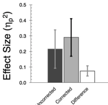
An additional 10 flavor, sensory preconditioning tests were subjected to this correction treatment and the effects on effect size and sample requirement examined. Some data came from unpub-lished observations; others came from pubunpub-lished data (Ward-Robinson, Coutureau, Good, Honey, Killcross, & Oswald, 2001; Robinson, Coutureau, Honey, & Killcross, 2005; Ward-Robinson et. al., 1998; Ward-Ward-Robinson, Wilton, Muir, Honey, Vann, & Aggleton, 2002). Figure 6 summarizes changes in the effect sizes and in the sample requirements of these experiments when data were in their original, uncorrected form and in their corrected form. The raw data are available in the supplemental materials. Although the effect size statistics were quite variable there was an apparent increase when the correction method was applied,t(10)⫽4.1,p⬍.003,p2⬎.625, 90% CI [.21, .76].
Cor-relation Coefficients, supported that description of the Cor-relationship for both the Kamin method,r(10)⫽ ⫹.91,p⬍.001, and for the Pfautz method,r(10)⫽ ⫹.81,p⬍.001.
Discussion
In general, the correction ratio offset the unwanted bias in flavor preference and improved the sensory preconditioning effect-size. The sensory preconditioning experiments varied in the extent of the flavor bias: In some there was a marked preference for sucrose over saline but in others there was none. The improvement in effect size was commensurate with the magnitude of the flavor bias: In experiments with large flavor biases, the correction ratio gave a correspondingly large improvement in the sensory precon-ditioning effect size; when there was no marked flavor bias, the ratio had no appreciably influence on the sensory preconditioning effect size.
The correction ratio also resolves a problem affecting the deci-sion to use stimuli from the same or from different modalities in discrimination tasks. One could assist discrimination by selecting stimuli from different modalities (e.g., a tone and a light in an appetitive discrimination with rats). However, such perceptually distinct stimuli often elicit different patterns of unconditioned response that differ in modifying the measured response (e.g., Jacobs & LoLordo, 1977) and may encourage selection in intra-modal stimuli (e.g., a tone and a clicker). One solution is, thus, to
facilitate discrimination by the selection of stimuli from different modalities before offsetting unwanted variation with the correction ratio.
The sensory preconditioning examples summarize here were taken from within-subjects experiments in which fluid consump-tion was measured. Of course, this correcconsump-tion ratio could be applied elsewhere to different experimental procedures with alter-native stimuli and measurement variables. For example, George and Pearce (1999) reported an experiment that suffered from an unwanted difference in the discriminability of two types of coun-terbalanced stimuli. In other regards, their experiment was quite different from the sensory preconditioning experiments: It used a between-subjects design, an autoshaping procedure with pigeons and a Kamin discrimination-ratio dependent variable, which was based on peck rates during reinforced and nonreinforced keylight stimuli. Two groups of pigeons received either an intradimensional shift or an extradimensional shift. The dimensions were colors and orientations, which were combined as keylight stimuli. For some of the intradimensional shift pigeons color was relevant to rein-forcement and orientation was irrelevant; for the remainder, ori-entation was relevant and color irrelevant to reinforcement. The same counterbalancing arrangement was applied to the extradi-mensional shift pigeons to permit meaningful comparison of the performance across intra-/extradimensional shifts. George and Pearce’s intradimensional pigeons out-performed the extradimen-Table 2
Raw and Transformed Consumption of Two Flavored Solutions
Flavor
A⫹ A⫹
Flavor
B⫺ B⫺
Uncorrected data
Corrected data
Uncorrected data
Corrected data
Sucrose 2 g 1.5 g Saline 23 g 34.8 g
Sucrose 7 g 5.2 g Saline 22 g 33.3 g
Sucrose 11 g 8.2 g Saline 17 g 25.7 g
Sucrose 12 g 9.0 g Saline 22 g 33.3 g
Sucrose 14 g 10.5 g Saline 14 g 21.2 g
Sucrose 14 g 10.5 g Saline 15 g 22.7 g
Sucrose 25 g 18.7 g Saline 2 g 3.0 g
Sucrose 25 g 18.7 g Saline 9 g 13.6 g
Saline 5 g 7.6 g Sucrose 19 g 14.2 g
Saline 0 g .0 g Sucrose 19 g 14.2 g
Saline 16 g 24.2 g Sucrose 19 g 14.2 g
Saline 3 g 4.5 g Sucrose 21 g 15.7 g
Saline 0 g .0 g Sucrose 22 g 16.4 g
Saline 5 g 7.6 g Sucrose 22 g 16.4 g
Saline 1 g 1.5 g Sucrose 22 g 16.4 g
Saline 0 g .0 g Sucrose 29 g 21.7 g
Saline 0 g .0 g Sucrose 29 g 21.7 g
Mean uncorrected sucrose consumption: 18.4 g Mean corrected sucrose consumption: 13.7 g Mean uncorrected saline consumption: 9.1 g Mean corrected saline consumption: 13.7 g Mean uncorrected overall consumption: 13.7 g Mean corrected overall consumption: 13.7 g Sucrose correction ratio: 13.7/18.4⫽.7 Sucrose correction ratio: 13.7/13.7⫽1 Saline correction ratio: 13.7/9.1⫽1.5 Saline correction ratio: 13.7/13.7⫽1
[image:9.603.48.555.99.349.2]sional pigeons but that effect was masked by the tendency in the two subgroups within each main group to learn more quickly if their relevant dimension was color, rather than orientation (see also, Mackintosh & Little, 1969; Urcuioli & Zentall, 1986).
Despite these differences from the sensory preconditioning pro-cedure examined above, the correction ratio may be applied in the same way to George and Pearce’s (1999) data. For example, by the fifth session that George and Pearce present in their Figure 2, intra-and extradimensional ratios are, respectively, 0.984 intra-and 0.933 in pigeons whose relevant dimension was color and 0.822 and 0.690 in pigeons whose relevant dimension was orientation. The bias in discrimination between color and orientation can be offset in the same way as for sensory preconditioning by the multiplication of each discrimination ratio by the appropriate correction ratio. The denominator for color correction ratio will be the average color discrimination ratio (i.e., (0.983⫹0.933)/2⫽0.958). The denom-inator for the orientation correction ratio will be the average orientation discrimination ratio (i.e., (0.822⫹0.690)/2⫽0.811). Both ratios’ numerator will be the overall average (i.e., (0.983⫹
0.933 ⫹ 0.822 ⫹ 0.690)/4 ⫽ 0.857). This produces a pair of
correction ratios for color-relevant discrimination ratios, 0.894 (i.e., 0.857/0.958) and orientation-relevant ratios 1.134 (i.e., 0.857/0.811) for multiplication with the corresponding, original discrimination ratio. Notice that birds’ superior performance on the color discrimination will be reduced because the correction ratio is⬍1 and that their inferior performance on the orientation dis-crimination will be boosted because its ratio is⬎1. This process could be repeated to create session-specific correction ratios, which would best accommodate variation in the color-orientation bias as the discrimination changes with training.
The correction ratio may also be expanded to include more than a pair of stimuli. For example, a sensory preconditioning test could include some third comparison flavor (e.g., umami), that would be counterbalanced across treatments with sucrose and saline. A third correction ratio with the denominator based on the mean uncor-rected umami consumption, irrespective of stimulus role, would be
used to correct the umami consumption data. The three flavors would have their own correction ratio with the overall average consumption as the numerator and the average consumption of that particular flavor as the denominator.
Where multiple nuisance variables (e.g., overall differences in performance in different operant chambers; unwanted sex differ-ences, etc.) affect the primary measurement, multiple correction ratios can be employed. For example, if George and Pearce had found that discrimination ratios varied across their eight Skinner boxes, they could compute correction ratios for each of the eight boxes and apply them appropriately to each bird’s data. This could be done in addition the correction for color-orientation bias. In this case the box and color-orientation biases would be corrected in equal measure. Of course, the influence of the two variables is unlikely to be equal and it may be preferable to weight each set of correction ratios before their application to the original data.
It is important to note that the correction ratio will not always improve effect size. In the sensory preconditioning examples the correction ratio selectively improved effect sizes when there was a sucrose-saline bias; when there was no bias, the correction ratio produced no effect-size improvement. However, there was no circumstance in which the sensory preconditioning data produced a smaller effect size after application of the correction ratio. However, there are circumstances in which this will happen. For example, the data in Table 1 summarize an improvement in effect size when the correction ratio is applied to sensory preconditioning data that are affected by a sucrose preference, relative to saline (p2⫽.379 increases top2⫽.493). Furthermore, if, for example, the consumption of B (saline) for the first rat of 23gis replaced with the value of 100 g, the effect size decreases fromp2⫽.280 top2⫽.266. These two observations demonstrate that the
[image:10.603.76.255.75.249.2]correc-Figure 6. Mean effect sizes (p2) for 11 sensory preconditioning experi-ments using sucrose or saline as test flavors. Data are in their original form (“Uncorrected”) or when subject to the correction treatment (“Corrected”). The third column summarizes values of the corrected minus the uncor-rected effect size statistics. Error bars represent 90% confidence intervals.
[image:10.603.334.517.438.616.2]tion ratio acts only where there is a systematic bias and will not provide an arbitrary improvement to effect size.
General Discussion
I examined two different ways of improving effect sizes in experimental data. One led us to examine the influence of discrim-ination ratios on effect size; the other used a correction ratio to offset the influence of a nuisance variable that may otherwise diminish effect size. The findings suggest that the Pfautz ratio (Pfautz et al., 1978) is preferred over the Kamin ratio (1969), which is similar to the Redhead (Redhead & Curtis, 2013; Redhead & Pearce, 1998) and Ennaceur (e.g., Ennaceur & Delacour, 1988) ratios. The correction ratio was seen to help effect size only when the nuisance variable had appreciable effect. We also saw that the application of correction ratios was general and fully expandable being applicable to variables with multiple levels and to (weighted) combinations of variables (such as differences in dis-crimination across stimulus dimensionandSkinner box).
The focus on effect size is only one side of the benefits of the sensible application of ratios to experimental data. An alternative, but inextricably related, consideration is for theNrequirements to reach a particular effect size. From a statistical point of view, larger Ns are always favored, but increasing N has unwanted impact on time and on resources costs. Such concerns are espe-cially acute in animal research where professional (e.g., American Psychological Association, 2012; The British Psychological Soci-ety, 2012), and legal (e.g., European Union, 2010; Home Office, 2013) responsibilities act to reduce the number of animals used in experimental work. Thus, the methods described here may con-tribute to meaningful reductions in animal requirement in experi-mentation in addition to improvements in effect size sensitivity.
References
American Psychological Association. (2012).Guidelines for ethical con-duct in the care and use of nonhuman animals in research. Retrieved from http://www.apa.org/science/leadership/care/guidelines.aspx Bonardi, C., & Jennings, D. (2009). Learning about associations: Evidence
for a hierarchical account of occasion setting.Journal of Experimental Psychology: Animal Behavior Processes, 35, 440 – 445. http://dx.doi .org/10.1037/a0014019
Cumming, G. (2011).Understanding the new statistics: Effect sizes, con-fidence intervals, and meta-analysis. London, United Kingdom: Taylor & Francis Ltd.
Ennaceur, A., & Delacour, J. (1988). A new one-trial test for neurobio-logical studies of memory in rats. 1: Behavioral data.Behavioural Brain Research, 31,47–59. http://dx.doi.org/10.1016/0166-4328(88)90157-X European Union. (2010).Directive 2010/63/EU of the European Parlia-ment and of the Council of 22 September 2010 on the protection of animals used for scientific purposes. Retrieved from http://eur-lex .europa.eu/legal-content/EN/TXT/?qid⫽1469445744396&uri⫽ CELEX:32010L0063
George, D. N., & Pearce, J. M. (1999). Acquired distinctiveness is con-trolled by stimulus relevance not correlation with reward.Journal of Experimental Psychology: Animal Behavior Processes, 25, 363–373. http://dx.doi.org/10.1037/0097-7403.25.3.363
Harris, J. A., Shand, F. L., Carroll, L. Q., & Westbrook, R. F. (2004). Persistence of preference for a flavor presented in simultaneous com-pound with sucrose.Journal of Experimental Psychology: Animal Be-havior Processes, 30,177–189. http://dx.doi.org/10.1037/0097-7403.30 .3.177
Hoffman, H. S., Selekman, W., & Fleshler, M. (1966). Stimulus aspects of aversive controls - long term effects of suppression procedures.Journal of the Experimental Analysis of Behavior, 9,659 – 662. http://dx.doi.org/ 10.1901/jeab.1966.9 – 659
Home Office. (2013).Guidance on the operation of the animals (Scientific Procedures) act 1986. Retrieved from https://www.gov.uk/government/ publications/operation-of-aspa
Howell, D. C. (2002).Statistical methods for psychology(5th ed.). Pacific Grove, CA: Duxbury.
Jacobs, W. J., & LoLordo, V. M. (1977). The sensory basis of avoidance responding in the rat: Relative dominance of auditory or visual warning signals and safety signals.Learning and Motivation, 8,448 – 466. http:// dx.doi.org/10.1016/0023-9690(77)90045-5
Kamin, L. J. (1969). Predictability, surprise, attention, and conditioning. In B. A. Campbell & R. M. Church (Eds.), Punishment and aversive behavior(pp. 279 –296). New York, NY: Appleton-Century-Crofts. Kelley, K. (2007). Confidence intervals for standardized effect sizes:
Theory, application, and implementation. Journal of Statistical Soft-ware, 20,1–24. http://dx.doi.org/10.18637/jss.v020.i08
Lakens, D. (2013). Calculating and reporting effect sizes to facilitate cumulative science: A practical primer for t-tests and ANOVAs. Fron-tiers in Psychology, 4,863. http://dx.doi.org/10.3389/fpsyg.2013.00863 Mackintosh, N. J., & Little, L. (1969). Intradimensional and extradimen-sional shift learning by pigeons.Psychonomic Science, 14,5– 6. http:// dx.doi.org/10.3758/BF03336395
Miller, R. R., Laborda, M. A., Polack, C. W., & Miguez, G. (2015). Comparing the context specificity of extinction and latent inhibition. Learning & Behavior, 43,384 –395. http://dx.doi.org/10.3758/s13420-015-0186-x
Montuori, L. M., & Honey, R. C. (2016). Perceptual learning with tactile stimuli in rats: Changes in the processing of a dimension.Journal of Experimental Psychology: Animal Learning and Cognition, 42,281– 289. http://dx.doi.org/10.1037/xan0000104
Pezze, M. A., Marshall, H. J., & Cassaday, H. J. (2016). Potentiation rather than distraction in a trace fear conditioning procedure. Behavioural Processes, 128,41– 46. http://dx.doi.org/10.1016/j.beproc.2016.04.003 Pfautz, P. L., Donegan, N. H., & Wagner, A. R. (1978). Sensory
precon-ditioning versus protection from habituation.Journal of Experimental Psychology: Animal Behavior Processes, 4,286 –295. http://dx.doi.org/ 10.1037/0097-7403.4.3.286
Redhead, E. S., & Curtis, C. (2013). Common elements enhance or retard negative patterning discrimination learning depending on modality of stimuli.Learning and Motivation, 44,46 –59. http://dx.doi.org/10.1016/ j.lmot.2012.05.001
Redhead, E. S., & Pearce, J. M. (1998). Some factors that determine the influence of a stimulus that is irrelevant to a discrimination.Journal of Experimental Psychology: Animal Behavior Processes, 24, 123–135. http://dx.doi.org/10.1037/0097-7403.24.2.123
Rescorla, R. A., & Cunningham, C. L. (1978). Within-compound flavor associations. Journal of Experimental Psychology: Animal Behavior Processes, 4,267–275. http://dx.doi.org/10.1037/0097-7403.4.3.267 Robinson, J., Sanderson, D. J., Aggleton, J. P., & Jenkins, T. A. (2009).
Suppression to visual, auditory, and gustatory stimuli habituates nor-mally in rats with excitotoxic lesions of the perirhinal cortex.Behavioral Neuroscience, 123,1238 –1250. http://dx.doi.org/10.1037/a0017444 Robinson, J. Whitt, E. J., Horsley, R. R., & Jones, P. M. (2010).
Familiarity-based stimulus generalization of conditioned suppression in rats is dependent on the perirhinal cortex.Behavioral Neuroscience, 124, 587–599. http://dx.doi.org/10.1037/a0020900
The British Psychological Society. (2012).Guidelines for psychologists working with animals. Retrieved from http://www.bps.org.uk/system/ files/images/animals_policy_statement.pdf
Urcuioli, P. J., & Zentall, T. R. (1986). Retrospective coding in pigeons’ delayed matching-to-sample.Journal of Experimental Psychology: An-imal Behavior Processes, 12, 69 –77. http://dx.doi.org/10.1037/0097-7403.12.1.69
Ward-Robinson, J., Coutureau, E., Good, M., Honey, R. C., Killcross, A. S., & Oswald, C. J. P. (2001). Excitotoxic lesions of the hippocampus leave sensory preconditioning intact: Implications for models of hip-pocampal function.Behavioral Neuroscience, 115,1357–1362. http://dx .doi.org/10.1037/0735-7044.115.6.1357
Ward-Robinson, J., Coutureau, E., Honey, R. C., & Killcross, A. S. (2005). Excitotoxic lesions of the entorhinal cortex leave gustatory within-event learning intact.Behavioral Neuroscience, 119,1131–1135. http://dx.doi .org/10.1037/0735-7044.119.4.1131
Ward-Robinson, J., & Hall, G. (1999). The role of mediated conditioning in acquired equivalence.The Quarterly Journal of Experimental Psy-chology, 52,335–350. http://dx.doi.org/10.1080/027249999393031 Ward-Robinson, J., Symonds, M., & Hall, G. (1998). Context specificity of
sensory preconditioning: Implications for processes of within-event
learning.Animal Learning & Behavior, 26,225–232. http://dx.doi.org/ 10.3758/BF03199215
Ward-Robinson, J., Wilton, L. A. K., Muir, J. L., Honey, R. C., Vann, S. D., & Aggleton, J. P. (2002). Sensory preconditioning in rats with lesions of the anterior thalamic nuclei: Evidence for intact nonspatial ‘relational’ processing. Behavioural Brain Research, 133, 125–133. http://dx.doi.org/10.1016/S0166-4328(01)00465-X
Whitt, E. J., Haselgrove, M., & Robinson, J. (2012). Indirect object recognition: Evidence for associative processes in recognition memory. Journal of Experimental Psychology: Animal Behavior Processes, 38, 74 – 83. http://dx.doi.org/10.1037/a0025886
Whitt, E., & Robinson, J. (2013). Improved spontaneous object recognition following spaced preexposure trials: Evidence for an associative account of recognition memory.Journal of Experimental Psychology: Animal Behavior Processes, 39,174 –179. http://dx.doi.org/10.1037/a0031344
Received February 1, 2017 Revision received May 2, 2017
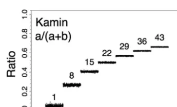
![Figure 5.A representation of the data summarized in Figure 4 that isconditions. The effect sizes are generally high because of the relativelypooled over the 3 SDs and the six varied conditional stimulus [CS]-rates.Mean effect sizes for one-sample ts that c](https://thumb-us.123doks.com/thumbv2/123dok_us/8583636.370097/7.603.73.257.76.226/figure-representation-summarized-isconditions-generally-relativelypooled-conditional-stimulus.webp)