Full Terms & Conditions of access and use can be found at
http://www.tandfonline.com/action/journalInformation?journalCode=pqje20
Download by: [University of Nottingham] Date: 24 July 2017, At: 03:46
The Quarterly Journal of Experimental Psychology
ISSN: 1747-0218 (Print) 1747-0226 (Online) Journal homepage: http://www.tandfonline.com/loi/pqje20
Learned Changes in Outcome Associability
Martyn C. Quigley, Carla J. Eatherington & Mark Haselgrove
To cite this article: Martyn C. Quigley, Carla J. Eatherington & Mark Haselgrove (2017): Learned Changes in Outcome Associability, The Quarterly Journal of Experimental Psychology, DOI: 10.1080/17470218.2017.1344258
To link to this article: http://dx.doi.org/10.1080/17470218.2017.1344258
Accepted author version posted online: 19 Jun 2017.
Submit your article to this journal
Article views: 16
View related articles
1
Publisher: Taylor & Francis & The Experimental Psychology Society
Journal: The Quarterly Journal of Experimental Psychology
DOI: 10.1080/17470218.2017.1344258
Learned Changes in Outcome Associability
Martyn C. Quigley, Carla J. Eatherington, Mark Haselgrove
The University of Nottingham
Correspondence Address:
School of Psychology
University of Nottingham
University Park
Nottingham, NG7 2RD, U.K.
2
Abstract
When a cue reliably predicts an outcome, the associability of that cue will change.
Associative theories of learning propose this change will persist even when the same cue is
paired with a different outcome. These theories, however, do not extend the same privilege to
an outcome; an outcome’s learning history is deemed to have no bearing on subsequent new
learning involving that outcome. Two experiments were conducted which sought to
investigate this assumption inherent in these theories using a serial letter-prediction task. In
both experiments participants were exposed, in Stage 1, to a predictable outcome (‘X’) and an
unpredictable outcome (‘Z’). In Stage 2 participants were exposed to the same outcomes
preceded by novel cues which were equally predictive of both outcomes. Both experiments
revealed that participants’ learning toward the previously predictable outcome was more
rapid in Stage 2 than the previously unpredicted outcome. The implications of these results
for theories of associative learning are discussed.
3
When a predictive relationship is arranged between two stimuli, an association
between these stimuli is assumed to be formed (e.g. Mackintosh, 1974, 1983; Pavlov, 1927;
Rescorla, 1968). In order to explain the mechanisms underpinning the formation and
subsequent modification of this association, a variety of formal learning models have been
devised (see: Pearce & Bouton, 2001, for review). Generally, these models can be categorised
into two types: unconditioned stimulus (US) processing models, and conditioned stimulus
(CS) processing models. According to the first class of these models, the US is capable of
supporting a finite amount of associative strength which is divided amongst the CSs, or cues,
presented prior to the presentation of a US, or an outcome.1 One of the most influential of
these models was proposed by Rescorla and Wagner (1972). This model states that the
change in the associative strength of a stimulus (∆V) is determined by the following equation:
∆
= α
β
(
λ
-
∑ )
(1)
Where α and β are learning rate parameters for the cue and the outcome, respectively,
which are fixed, and are determined by the salience of these two stimuli; λ represents the
maximum amount of conditioning supported by the outcome, and ∑V is the summed
associative strength of all cues present on a trial. Informally, the model proposes that
associative learning will be most effective between cues and outcomes that are
unconditionally salient and, in particular, when the outcome is unexpected – and hence better
processed.
Alternatively, CS processing models or “attentional models”, assume that the
predictability of a cue influences its associability (i.e. the extent to which it enters into
1The terms cue and conditioned stimulus (CS), and outcome and unconditioned stimulus (US) are
4
associations). One of the most influential of these models was proposed by Mackintosh
(1975). Within this model, henceforth the ‘Mackintosh model’, the change in the associative
strength of a stimulus e.g. ‘A’ (∆ A) is determined by the following equation:
∆
A=
α
Aβ
(
λ
-
V
A)
(2)
Here, A refers to the associability of stimulus A, β is, again, a fixed learning-rate
parameter determined by the salience of the outcome, and λ the asymptotic value of learning
possible on that trial. Crucially, within this model the parameter α is deemed to alter as a
function of experience: Stimulus A will gain in associability if it is a better predictor of an
outcome than all other stimuli present on a given trial, otherwise the associability of A will
decrease. These rules can be expressed in the following formulae:
∆
A>
0
if
| −
A|
<
| −
r|
(3)
∆
A<
0
if
| −
A|
>
| −
r|
(4)
In which ∆ A is the change in the associability of stimulus A; λ − A is the difference
between the asymptotic value and the associative strength of stimulus A, and λ − r is the
discrepancy between the asymptotic value and the associative strength of all cues present on
that trial, apart from A (that is to say, the remainder).
A large body of evidence in both human (e.g. Bonardi, Graham, Hall, & Mitchell,
2005; Le Pelley & McLaren, 2003; Livesey & McLaren, 2007) and non-human animals (e.g.:
Haselgrove, Esber, Pearce & Jones, 2010; Mackintosh & Little, 1969) has supported the
5
demonstrated in humans by the ‘learned predictiveness’ effect. In a typical learned
predictiveness experiment, participants are exposed, in Stage 1, to a set of cues, some of
which are reliable predictors of an outcome and some of which are unreliable predictors of an
outcome. In Stage 2, these cues are arranged in a manner which makes them equally reliable
predictors of novel outcomes. What is typically observed in such experiments is a bias in
learning during Stage 2 to the cues that had greater predictive history in Stage 1; this effect is
apparent when the cues are presented in isolation (Le Pelley, Turnbull, Reimers & Knipe,
2010) or in compound with other cues (e.g. Le Pelley & McLaren, 2003).
An assumption inherent in the Mackintosh model, and which is demonstrated in
learned predictiveness experiments, is that variations in a cue’s associability will persist
despite the cue being separated from the outcome with which the cue was initially established
as either a good, or poor predictor. Thus, cue processing is, to a degree (Le Pelley, Oakeshott,
Wills & McLaren, 2005), independent of the outcome. Interestingly, however, this
independence of processing is not granted to the outcome. First, the learning rate parameter
for the outcome, β, is fixed, being determined only by its unconditioned properties (e.g. its
salience). Second, whilst the extent to which the outcome can support learning can change as
a function of how surprising it is (e.g. Rescorla & Wagner, 1972), this variation is dependent
on the presence of the cue which established the predictability of the outcome (e.g. λ-ΣV in
Equation 1). Hence, variations in outcome processing are deemed to be cue-dependent.
This approach is not unique to the Mackintosh model. Other, well established and
more recent hybrid models, (e.g. Esber & Haselgrove, 2011; Le Pelley, 2004; Pearce & Hall,
1980), also assume that learned variations in processing of the outcome is either non-existent
or cue-dependent. This assumption within these models appears reasonable, whilst it makes
sense for a cue to undergo changes in associability as a result of its predictive history, it is
6
predictability. When a cue is presented, for instance, it can signal the absence or presence of
an event, thus learning about the predictive nature of a cue is beneficial to an organism as it
allows the organism to anticipate the event. Yet, when an outcome is presented the event has
already happened, therefore it is difficult to see why a mechanism which mediates
associability changes of an outcome would be necessary.
Nevertheless, a number of phenomena within the learning literature have
demonstrated that prior experience with an outcome can influence subsequent behaviour
involving that outcome. For example, a number of studies within both the human and animal
literature have reported variations in the response produced by an outcome as a consequence
of how well-predicted it has been in the past (see Marcos & Redondo, 2001). Interestingly,
establishing an outcome as predictable has produced both diminution (i.e. attenuated
responses; see Kimble & Ost, 1961; Marcos & Redondo, 1999) and facilitation (i.e. enhanced
responding; see Donegan, & Wagner, 1987). A range of explanations have been provided for
these effects; typically, however, these explanations invoke variations in the effectiveness of
the outcome as a function of the presence (or absence) of the cue (λ-ΣV). Thus, no appeal to
any change in cue-independent variations in outcome processing has been required.
Additional phenomena within the learning literature have also suggested that exposure
to an outcome can influence subsequent learning involving that outcome. One such
phenomenon is the US pre-exposure effect, where exposure to the US, prior to CS-US
pairings, impairs subsequent learning supported by that US (e.g. Kremer, 1971; see Randich
& LoLordo, 1979, for review). This effect has been demonstrated in humans (Taylor, 1956)
and rats (Kamin, 1961). This finding has been understood in terms of context blocking (e.g.
Baker & Mercier, 1982), according to which pre-exposure with the US results in the
formation of an association between the context and the US, permitting the context to
7
received much support (e.g. Baker & Mackintosh, 1979), however, notably, Baker and
Mercier (1982), came to the conclusion that whilst the context may mediate the US
pre-exposure effect, it is also conceivable that during pre-pre-exposure to the US, learning is acquired
regarding the unpredictable nature of the US, which influences subsequent learning in Stage 2
(See also: Randich & Lolordo, 1979). That is, the outcome is coded as unpredictable, thus
impairing the formation of predictive relationships (associations) between the CS and this US
at a subsequent stage. This latter explanation would seem to indicate that previous exposures
to the US could potentially change the associability of the outcome itself regardless of the
cue, or context, which it is was trained with.
Similarly, Baker and Mackintosh (1977) demonstrated that when a CS and US are
presented in an uncorrelated manner, these presentations impair subsequent conditioning
between the two stimuli. This ‘learned irrelevance’ effect has been accounted for by
assuming that these uncorrelated pre-exposures result in the CS and the US being deemed
‘irrelevant’ (e.g. Baker & Mackintosh, 1979). However, this interpretation has been
challenged. Matzel, Schachtman and Miller (1988) suggested that the deficit in learning is
underpinned by pre-exposure to the CS, pre-exposure to the US, and a learned irrelevance
effect. Furthermore, Bonardi and Ong (2003; also see Bonardi & Hall, 1996), in a review of
the literature, concluded that there is no evidence of a genuine learned irrelevance effect
above and beyond the effects of CS and US pre-exposure. The phenomena discussed above
imply that previous experience with an outcome can influence subsequent learning involving
that outcome. However, there is scant support for the idea that these changes in the extent to
which an outcome can support learning persist in the absence of the cue with which the
outcome was initially trained, or indeed beyond standard associative learning phenomena
(e.g. context blocking, or latent inhibition). To date, only one study, in humans, has explored
8
paired with this outcome. In this study, Griffiths, Mitchell, Bethmont, and Lovibond (2015)
adapted a food allergist procedure where participants were required to identify foods (i.e.
cues) that produced certain illnesses (i.e. outcomes). The results of this study revealed that
participants displayed impaired learning about an illness (i.e. the outcome) which had been
unreliably predicted in the past relative to an illness which had been well-predicted in the
past.
In light of the potential theoretical significance of the data reported by Griffiths et al.
(2015), the current experiments explored the generality of this effect with a serial
letter-prediction procedure, in which participants were tasked with learning the predictive
relationships between certain target letters. This experimental procedure has been
successfully used in a range of studies of learned variations of cue processing (e.g. Evans,
Gray & Snowden, 2007; Granger, Moran, Buckley & Haselgrove, 2016; Young, Kumari,
Mehrotra, Hemsley, Andrew, Sharma, Williams & Gray, 2005) and permits measurements of
learning derived from both rating scales and response times. The aim of the current
experiments was to assess whether the prior predictability of outcomes influenced the rate at
which they were learned about, when subsequently predicted by novel cues. If the associative
history of an outcome produces an effect comparable to a learned predictiveness effect, it
would be expected that a previously well-predicted outcome would be learned about more
readily than a previously less well-predicted outcome. Such a finding would constitute a
conceptual replication of the results reported by Griffiths et al. (2015) and a major challenge
9
Experiment 1
Experiment 1 comprised a serial letter-prediction task in which participants were
required to make a response to certain target letters or ‘outcomes’. The design of Experiment
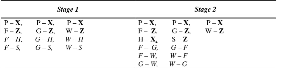
1 can be seen in Table 1.
---
TABLE 1 HERE
---
In Stage 1, letters X and Z were established as a predicted and a less
well-predicted target stimulus, respectively (referred to henceforth as the predicted outcome, and
the unpredicted outcome) and participants were asked to respond either upon their
presentation or beforehand if they thought they could anticipate their presentation. To
establish one letter (e.g. X) as a predicted outcome, this letter was only ever preceded by one
other letter (e.g. P). To establish an outcome as being unpredictable (e.g. Z), three letters (F,
G and W) preceded this outcome with equal frequency. In Stage 1 the letters F, G and W also
preceded the letters S and H an equal number of times. These trials, in which F, G and W
were paired with S and H, served three purposes. First, they ensured that the unpredicted
outcome was in fact unpredictable. Without these trials Z would merely have a greater
number of predictors. Second, these trials ensured that S and H (which would serve as cues
for X and Z in Stage 2) were familiarised to participants prior to the crucial test stage. And
third, these trials served as non-target trials during which participants were not required to
make a response.
Stage 2 followed seamlessly from Stage 1. Here, trials in which P was paired with X,
10
however, H and S were now paired equally frequently with X and Z respectively. The
question of central interest was whether participants would come to acquire a more rapid
response time to H (which was paired with the previously predicted outcome, X) than to S
(which was paired with the previously unpredicted outcome, Z). Additional non-target trials
11
Method
Participants
Thirty-two participants (18 Females; 14 Males) were recruited from the University of
Nottingham’s School of Psychology. Participants ranged from 19 – 51 years of age (M =
23.8; SEM = 1.40). All participants had normal or corrected-to-normal vision. Participants
received course credit for their participation. The study was conducted in accordance with the
British Psychological Society (2009) guidelines, receiving institutional ethical approval from
the University of Nottingham’s Psychology ethics committee.
Apparatus and Stimuli
All stimuli were presented (and responses recorded) in the graphical experimental
software package PsychoPy2, v1.82.02 (see Peirce, 2007; Peirce 2008), running on Windows
7 on a standard desktop computer. The stimuli were white capital letters, Arial [7mm × 5mm;
h × w], which appeared in the centre of the screen [27cm × 46cm; h × w] against a grey
background. The stimulus letters were, ‘F’, ‘G’, ‘H’, ‘P’, ‘S’ and ‘W’. The target stimuli [i.e.
the outcomes] were ‘X’ and ‘Z’. The actual stimulus letters which served as the cues,
outcomes, and non-target trials were counterbalanced across experimental versions using a
Latin-Squared counterbalancing technique. Stimulus letters never appeared simultaneously
on screen.
Procedure
All participants were tested individually. Once participants had provided their consent
they read the following instructions on screen before being exposed to Stage 1:
“Thank you for participating in this experiment.
In this experiment you will see individual letters appear in the centre of the screen.
It is your job to press X when you see X appear and press Z when you see Z appear. At first
12
continues, you might be able to anticipate when they are going to be presented. If you think
you know when either X or Z are going to appear, you can press them BEFORE they are
presented.
Please try to respond as quickly as you can when you think you know when X or Z are
going to appear. If you have no questions, please have your fingers ready over the X and the
Z, and then press the space bar to begin the experiment.”
Stage 1
In Stage 1, participants were exposed to 6 blocks of 12 trials (72 trials in total) in
which a trial constituted a pairing of two stimuli. Trial order was block randomised, and there
was no break between blocks. In each block participants received 3 pairings of P and X, 1
pairing each of F, G, and W with Z ; and 1 pairing each of F, G, and W with S and 1 pairing
each of F, G and W with H. Each trial lasted 4 seconds. On a target trial, for example, a cue
would be presented (e.g. P) for 1 second, followed by an inter-stimulus interval of 1 second,
an outcome (e.g. X) of 1 second, and finally a 1 second interval before the next cue was
presented (see Figure 1). In total, Stage 1 lasted 4.8 min. Once all 72 trials were complete,
Stage 2 began. There was no break between the two stages.
Stage 2
In Stage 2 participants were exposed to 18 blocks of 16 trials, the order of which was
randomised within each block. In this stage the trials which established the predictability of
the outcomes were carried over from Stage 1in order to make the two stages more similar.
Thus, in each block participants received 3 pairings of P and X and 1 pairing each of F, G,
and W with Z. In addition, H and S were each paired with the predicted and unpredicted
outcomes (e.g. X and Z) respectively, for two trials; and F, G and W were paired with each
13
---
FIGURE 1 HERE
---
Scoring and Error Classification
Response times could range from 0 – 3 seconds. Responses made between 0 – 1
seconds indicated that participants were responding during the presentation of the cue letter
(e.g. the letter P in a P–X pairing). Responses between 1 – 2 seconds indicated that
participants were responding during the inter-stimulus interval following the presentation of
the cue. Responses between 2–3 seconds indicated that participants were responding to the
outcomes as they were presented (X or Z). Response times were only analysed for P-X and
F/G/W-Z trials in Stage 1, and on H-X and S-Z trials in Stage 2. If participants omitted a
response (i.e. they failed to press the respective outcome key [e.g. X or Z] within the 0–3
second window) they were allocated a response time of 3 seconds for the trial. This type of
error was classed as an ‘omission’. If participants made an erroneous prediction (e.g. by
selecting the letter X when in fact Z was the outcome), they would also be allocated a
14
Results and Discussion
---
FIGURE 2 HERE
---
Response Time Data
Figure 2 shows the mean response time to the predicted and unpredicted outcomes in
Stage 1 across the 18 trials. The predicted stimulus refers to the outcome (e.g. X) which was
reliably paired with one cue (e.g. P); the unpredicted stimulus refers to the outcome (e.g. Z)
which was preceded by three letters (F/G/W). The response times for these data were collated
by looking at responses to the target stimuli within the 0-3 second window beginning
immediately upon the presentation of the cue that preceded the targets. Inspection of the data
reveals that as training progressed, response times for the predicted outcome shortened.
Furthermore, from Trial 6 onwards participants were, on average, responding to the outcome
prior to its presentation. In contrast, response times to the unpredicted outcome stayed
relatively constant across all 18 trials, with participants, on average, responding to the
outcome only during its presentation. This impression was confirmed with a 2 x 18 repeated
measures analysis of variance (ANOVA) of individual response times with the variables of
outcome (Unpredicted vs Predicted) and trial (1 – 18); in light of sphericity violations for the
“trial” variable, χ2 (152) = 259.55, p < .001 and the interaction between trial and outcome,
χ2 (152) = 215.50, p < .001, Greenhouse-Geisser values are reported.2 The ANOVA revealed
significant main effects of outcome, F (1, 31) = 20.71, MSE = 4.26, p = < .001, ηP2 = .40, and
2
15 trial, F (8, 253) = 13.48, MSE = .50, p = < .001, 2
P
η = .30, and a significant interaction
between the two variables, F (8, 259) = 6.12; MSE = .47, p = < .001, 2
P
η =.17. Simple
main-effects analyses revealed no significant differences between the outcomes for trials 1 - 4,
smallest, F (1, 31) = 2.27, MSE = .04, p = .14, but a significant difference for all other trials,
smallest F (1, 31) = 5.68, MSE = .51, p = .02.
---
FIGURE 3 HERE
---
Figure 3 shows the mean response times to the predicted and unpredicted outcomes in
Stage 2, on trials when the outcomes were reliably, and equivalently, predicted by cues H and
S. The data in Figure 3 have been collapsed into 9 blocks, each comprising 4 trials. In
keeping with Stage 1, the response time data for these analyses were collated by looking at
responses within the 0-3 second window following the onset of cue H or S. Figure 3
demonstrates that despite both outcomes initially producing similar mean response times on
the first block, response times to the previously predicted outcome became faster than the
previously unpredicted outcome. These impressions were confirmed with a 2 x 9 repeated
measures ANOVA of individual response times with the variables of outcome (unpredicted
vs predicted) and block (1 – 9), which revealed significant main effects of outcome, F (1, 31)
= 4.86, MSE = 1.54, p < .05, 2
P
η = .14, and block, F (4, 105) = 30.60, MSE = .46, p < .001, 2
P
η
= .50. The interaction between these variables was not significant, F (4, 115) = 2.05, MSE =
.31, p = .09, 2
P
η = .06. Overall, these results demonstrate that the previously predicted
16
Error Data
The mean percentage of errors for the predicted and the unpredicted outcome was
calculated for both Stage 1 and Stage 2. The Stage 1 error counts were calculated by
analysing the number of errors committed on the P–X trials for the predicted outcome and the
F/G/W–Z trials for the unpredicted outcome. Inspection of these data revealed that a
relatively low percentage of errors were committed for both the predicted outcome (M =
3.81%, SEM = 1.65) and the unpredicted outcome (M = 3.65%, SEM = 1.05). Participants
also made comparable percentages of omissions (M = 3.21%, SEM= .88) and commissions
(M = 4.25%, SEM = 1.82). A 2 × 2 repeated measures ANOVA of individual percent errors
with the variables of outcome (predicted vs unpredicted) and error type (omission vs.
commission) revealed no main effect of outcome, F (1, 31) = .01, MSE = 70.66, p = .91, 2
P
η =
.00, no effect of Error Type, F (1, 31) = .46, MSE = 75.54, p = .50 2
P
η = .02, and no
interaction between these two variables, F (1, 31) = .88, MSE = 69.69, p = .35 2
P
η = .03.
The Stage 2 error counts were calculated by analysing the number of errors
committed on the H – X and S – Z trials. Inspection of these data revealed that participants,
again, made relatively few errors for both the predicted (M = 5.56%, SEM = 1.87) and
unpredicted outcome (M = 4.03%, SEM = 1.12) in this stage. As in Stage 1, slightly more
commissions (M = 5.60%, SEM= 2.09) were committed than omissions (M = 3.99%, SEM=
.89). An identical ANOVA to that conducted upon the percentage error data from Stage 1
was conducted upon the data from Stage 2. This analysis revealed no main effect of outcome,
F (1, 31) = 1.77, MSE = 41.82, p = .19, 2
P
η = .05, no effect of error type, F (1, 31) = .55, MSE
= 151.04, p = .47 2
P
η = .02, and no interaction between these two variables, F (1, 31) = 1.22,
MSE = 35.87, p = .28 2
P
η = .04.
Experiment 1 demonstrated that establishing outcomes as differentially predicted,
17
Following learning about P–X and F/G/W–Z in Stage 1, participants displayed faster overall
learning to the predicted outcome (H–X) in Stage 2 than the unpredicted outcome (S–Z).
These results pose a challenge to attentional-theories of learning which do not grant an
independence of processing to outcomes (Esber & Haselgrove, 2011; Le Pelley, 2004;
Mackintosh, 1975; Pearce & Hall, 1980; Rescorla & Wagner, 1972). These models assume
that when a previously learned-about outcome is separated from the cue which established
the predictability of the outcome, the associative history of the outcome should not influence
subsequent learning. However, the results of Experiment 1 appear to contradict this
assumption.
18
Experiment 2
Although the results of Experiment 1 are consistent with the suggestion that outcomes
can come to acquire differential associability as a consequence of being either well or poorly
predicted in the past, it is possible to develop an alternative explanation for these results from
the perspective of standard associative models of learning. During Stage 1, participants were
given trials in which F, G and W, were each paired with Z: trials which may have resulted in
the establishment of excitatory associations between each of these stimuli and Z. On other
trials, F, G and W, are paired with H, and on other trials with S. Consequently, on these
F/G/W-H or F/G/W-S trials there may have been an expectation of the presentation of Z
which, importantly, was always unfulfilled. These circumstances are precisely those which
standard models of associative learning (e.g. Rescorla & Wagner, 1972) predict will result in
the establishment of an inhibitory association between H and Z, and S and Z. This inhibition
will then have to be overcome on trials in which S and Z are paired in Stage 2, before the
acquisition of excitatory associative learning between these stimuli can be expressed. Thus
the S-Z training will appear to be less successful than the H-X training, which was precisely
the result observed in Experiment 1. Experiment 2 sought to rule out this alternative
explanation for the results of Experiment 1, by arranging the stimuli in a manner which
would circumvent any differential inhibitory association being formed between the stimuli
which served as the test cues in Stage 2 (H and S) and the unpredicted outcome during Stage
1.
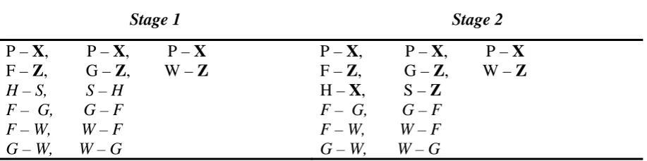
The strategy in Experiment 2 was to employ a design where H and S were never
preceded by F, G or W. Thus, there was no opportunity for an unfulfilled expectation of Z to
be present during trials featuring H and S, and consequently the establishment of inhibition.
We were, however, still keen to familiarise participants with H and S before they were
19
paired with each other in Stage 1 (i.e.: S–H and H-S). As in Experiment 1, non-target trials
were again formed by pairing the F, G and W stimuli with each other (as in Stage 2 of
Experiment 1). The full design of Experiment 2 can be seen in Table 2. If the effect observed
in Experiment 1 is still present using this design, this would suggest that any impaired
performance involving the unpredicted outcome in Stage 2 was not solely underpinned by an
inhibitory association between the previously unpredicted outcome (e.g. Z) and its novel cue
(e.g. S) during Stage 1 training. In addition, following completion of Stage 2, a set of rating
scales were presented which required participants to rate how predictive each stimulus was of
the target stimuli (X and Z). If these scales are consistent with the response time data in
Experiment 1, it would be expected that the cue (S) which was paired with the previously
unpredicted outcome (Z), would be rated as being less predictive than the cue (H) which was
paired with the previously predicted outcome (X).
---
TABLE 2 HERE
20
Method
Participants
Thirty-two participants (29 Females; 3 Males) were recruited from the University of
Nottingham’s School of Psychology. Participants ranged from 18 – 46 years of age (M =
20.2; SEM = 0.89). Participants received course credit for their participation. A cash prize of
£10 was also awarded to the participant who completed the experiment with the fastest
overall reaction time on trials where the target stimuli were present. All other details were the
same as in Experiment 1.
Apparatus and Stimuli
The apparatus and stimuli for Experiment 2 were identical to Experiment 1. However
once Stage 2 had been completed participants were presented with two ratings screens, one
for each of the target stimuli (X and Z). These screens requested participants provide a rating
for each stimulus’s (i.e. ‘F’ ‘G’ ‘H’ ‘P’ ‘S’ and ‘W’) ability to predict the absence or presence
of the target stimuli on a scale ranging from ‘-100’ to ‘+100’ [‘-100’ = ‘Predicts absence of
target stimulus’; ‘0’ = ‘Don’t Know’ ‘+100’ = ‘Predicts presence of target stimulus’]. Six
rating scales for each of the letters appeared on the same screen at the same time, for each
rating screen. Each of the six scales was placed alongside each of the respective letters.
Procedure
The procedure for Experiment 2 was identical to Experiment 1, with the exception
that the letters (H and S) which would serve as cues for X and Z in Stage 2 were paired with
each other in Stage 1 twice per block (i.e. H–S, S–H). Thus, these pairings were presented a
total of 12 times across Stage 1. Within Stage 1, the stimuli F, G and W, were also paired
with each other to form non-target trials (e.g. F–G, F–W, G–F, G–W, W–F and W-G), as in
21
presented a total of 36 times across Stage 1. In total Stage 1 lasted 5.6 mins. The procedure
for Stage 2 was identical to Stage 2 of Experiment 1.
Once participants had completed Stage 2 they were presented with the following text:
“Thank you. The experiment is nearly complete. Before finishing, however, there are a few
questions to complete. Please press the ‘SPACEBAR’ to proceed.” Participants were then
presented with a rating screen for each of the target stimuli (X and Z). Participants then
provided a score ranging from -100 to + 100 regarding how predictive of the absence or
presence of X or Z each other letter was. Participants provided their score by adjusting a tick
maker on a scale. The numerical value of the tick marker position was provided in a grey box
22
Results and Discussion
---
FIGURE 4 HERE
---
Response Time Data
Figure 4 shows the mean response time to the predicted and unpredicted outcomes in
Stage 1 across the 18 trials. In keeping with Experiment 1, the response times for these data
were collated by looking at responses within the 0 – 3 second window beginning with the
presentation of the cue. Inspection of the data presented in Figure 4 reveals that as training
progressed, response times for the predicted outcome shortened. Furthermore, Figure 4
demonstrates that from Trial 7 onward participants were, on average, responding to the
predicted outcome before its presentation. In contrast, response times to the unpredicted
outcome stayed relatively constant across all 18 trials, with participants, on average,
responding to the outcome only when the outcome had been presented.
A 2 x 18 repeated measures ANOVA was performed on these data with the variables
of outcome (Unpredicted vs Predicted) and trial (1 – 18). The ANOVA revealed significant
main effects of outcome, F (1, 31) = 55.23, MSE = 2.19, p = < .001, 2
P
η = .64, and trial, F (8,
247) = 15.5, MSE = .40, p = < .001, 2
P
η = .34, and a significant interaction between these
variables, F (8, 242) = 10.74, MSE = .40, p = < .001, 2
P
η =.26. Simple main-effects analyses
revealed significant differences between the outcomes (ps < .05) from Trial 2 onward,
23
---
FIGURE 5 HERE
---
Figure 5 shows, over 9 four-trial blocks, the mean response times to the predicted and
unpredicted outcomes in Stage 2, on trials when the outcomes from Stage 1were both reliably
and equivalently predicted by cues H and S. In keeping with Experiment 1, response times
were similar for both the previously predicted and unpredicted outcomes at the outset of
Stage 2. However, overall, response times to the previously predicted outcome from Stage
1were faster than the unpredicted outcome from Stage 1.
A 2 x 9 repeated measures ANOVA was performed on these data with the variables of
outcome (Unpredicted vs Predicted) and block (1 – 9). The ANOVA revealed significant
main effects of outcome, F (1, 31) = 8.08, MSE = 1.56, p < .01, 2
P
η = .21, and block, F (3,
92) = 41.54, MSE = .57, p < .001, 2
P
η = .57. The interaction effect between the two factors
approached significance, F (3, 106) = 2.34, MSE = .28, p = .07, 2
P
η = .07. For the curious
reader, simple main effects analyses were conducted to identify the source of the interaction
which approached significance. These analyses revealed significant differences between the
outcomes (ps < .05) on Blocks 2 - 7. There were no significant differences on blocks 1, 8 or
9,largest F (1, 31) = 2.79, p = .11.
Error Data
As in Experiment 1, the mean percentage of errors for the predicted and the
unpredicted outcome was calculated for both Stage 1 and Stage 2 data. Inspection of the data
from Stage 1 revealed that participants made more errors for the unpredicted outcome (M =
5.82, SEM = 1.31) than the predicted outcome (M = 3.56, SEM = 1.16) and more
24
impressions were largely confirmed with a 2 × 2 repeated measures ANOVA of percentage of
errors with the variables of outcome (unpredicted vs predicted) and error type (commission
vs omission). The ANOVA revealed a main effect of outcome F (1, 31) = 6.2, MSE = 24.61,
p = .02, 2
P
η = .18. The main effect of error type approached significance, F (1, 31) = 3.42,
MSE = 81.62, p = .07, 2
P
η = .10. There was no significant interaction between these two
factors, F (1, 31) = .118; MSE = 32.73, p = .73, 2
P
η =.00.
Inspection of the Stage 2 data revealed that participants made a comparable number of
errors for the predicted outcome (M = 5.43, SEM= 1.45) and the unpredicted outcome (M =
4.69, SEM = 1.68), with more commissions (M = 6.90, SEM = 1.62) than omissions (M =
3.21, SEM = 1.51). An identical ANOVA to that conducted on the error data from Stage
1was conducted on the Stage 2 data which revealed a main effect of error type, F (1, 31) =
4.83, MSE = 90.17, p = .04, η2P= .14, but no effect of outcome F (1, 31) = 1.31, MSE = 13.31,
p = .26, ηP2= .04, and no interaction, F (1, 31) = .08, MSE = 61.75, p = .78,
2
P
η = .00.
---
FIGURE 6 HERE
25
Rating Data
Figure 6 shows participants’ ratings of how predictive they deemed each of the cues
to be for the target outcomes (X or Z). The ratings for the three stimuli paired with the
unpredicted outcome in Stage 1 (e.g. ‘F’, ‘G’, ‘W’) were collapsed by averaging the values
for these stimuli. Four participants failed to provide ratings, either omitting some or all of the
rating scales; an additional participant was removed as their ratings were more than 3
standard deviations above the mean (Z score > 3.27), closer inspection of their ratings
indicated they used the scale in the opposite manner in which it was intended. Thus, a total of
5 participants were omitted from the subsequent analyses (n = 27).
As can be seen in Figure 6, the ‘P–X’ ratings and ‘H–X’ ratings were comparably
high, and both higher than the ‘S–Z’ rating. The three stimuli (‘F/G/W’) paired with the
unpredicted outcome (‘Z’) received only a mildly positive rating. A repeated measures
one-way ANOVA of individual ratings with four levels (P–X, F/G/W–Z, H–X, and S–Z) was
significant, F (2, 56) = 41.62, MSE = 2074.94, p < .001, 2
P
η = .62. Planned comparisons using
Bonferonni corrected t-tests (adjusted p = .025) revealed a significant difference between the
predictiveness ratings for the stimulus pairings P-X and F/G/W – Z, t(26) = 9.01, p <. 001,
and a significant difference between H–X and S–Z, t(26) = 2.86, p <. 01. These results
corroborate the response time data from Stage 2: participants were biased towards learning
about the cue paired with the previously predicted outcome (H–X) relative to the cue paired
with the previously unpredicted outcome (S–Z).
Experiment 2 replicated and extended the findings of Experiment 1, again
demonstrating that the previous predictability of an outcome influences the rate at which it is
subsequently learned about when signaled by a cue which it has not previously been paired
with. These results were obtained using an experimental design that ruled out the contribution
26
keeping with Experiment 1, the Stage 2 error data indicates the difference in the response
time data is not undermined by a speed-accuracy trade off as both outcomes produced a
comparable (and relatively low) number of errors; thus indicating that whilst participants are
able to learn the association involving the previously unpredicted outcome, the previously
predicted outcome enters into associations more readily. The rating data corroborate this.
Although both cues for the outcomes from stage 2 received positive ratings, participants
provided higher ratings to the cue paired with the previously predicted outcome, than the cue
that was paired with the previously unpredicted outcome.
General Discussion
Two experiments investigated whether an outcome’s prior associative history
influences subsequent learning involving that outcome, when separated from the cue with
which the outcome was first paired with. In both experiments, participants displayed a bias in
learning towards a previously predicted outcome, with the predicted outcome entering into
associations with novel cues more readily than the previously unpredicted outcome. Although
Experiment 1 could be accounted for by appealing to the role of inhibitory learning
established in Stage 1, the design of Experiment 2 ruled out this explanation, and replicated
the effect observed in Experiment 1 both with response time measures and, in addition,
self-report ratings.
These results are consistent with the findings of Griffiths et al. (2015) supporting their
notion of a “learned predictability” effect within outcomes. In their study, Griffiths et al.
(2015), employed a procedure in which participants were required to take on the role of a
food allergist and identify which symptoms followed the consumption of certain foods in
27
of foods (AX and BX) were followed by two different types of outcomes (e.g. Stomach
Reaction and Skin Rash), which each comprised a compound of symptoms. The outcome
Stomach Reaction consisted of the symptoms cramping and bloating, whilst the outcome
Skin Rash consisted of the symptoms itchiness and swelling. One outcome’s symptoms
would be well-predicted (e.g. Stomach Reaction), with each of its symptoms (e.g. cramping
and bloating) reliably predicted by cues A and B, whilst the other outcome’s symptoms (e.g.
Skin Rash) would be less well-predicted, as cue X was equally predictive of either symptom.
In Stage 2, novel cues (E, F, G, H) were reliably paired with the previously less
well-predicted symptom of an outcome and the previously well-well-predicted symptom of an outcome,
and participants were required to predict the symptoms produced by the cues. The results
demonstrated that participants better learned associations involving the previously
wellpredicted outcome’s symptoms than the previously less wellwellpredicted outcome’s symptoms
-a result consistent with the d-at-a from the two experiments reported here.
Interestingly, two other studies may also be of relevance when considering the
prospect of learned variations in outcome processing, both of which seemingly demonstrate a
blocking effect among the components of an outcome. In a typical blocking procedure,
pre-training one component (A+) of a compound (AB+) impairs learning to the added cue (B) of
the compound in a subsequent test (Kamin, 1968, 1969). However, in a series of experiments
investigating second-order conditioning, Rescorla (1980, p 91- 97) investigated possible
interactions among aspects of a reinforcer (or an outcome) and demonstrated blocking in an
outcome. In the particular experiment of interest, pigeons were exposed to intermixed
presentations of a cue (A) being paired with both a single outcome (‘O1’) and a compound
outcome (‘O1 + O2’). As a result of these trials the pigeons demonstrated weak learning
about the A-O2 association relative to a control group who received comparable treatment,
28
outcome compete for associative strength in the same manner as cues (see also: Miller &
Matute, 1998 for a similar demonstration with rats).
Thus, the current experiments, together with others (Griffiths et al., 2015; Rescorla,
1980; Miller & Matute, 1998) suggest that a revision may be required to learning models
which stipulate that β is a fixed learning-rate parameter. It is thus tempting to suggest that
changes in attention/associability to both cues (α) and outcomes (β) are underpinned by
comparable rules. For example, the algorithms suggested by Mackintosh (1975; see also:
Esber & Haselgrove, 2011; George & Pearce, 2012; Le Pelley, 2004), for changes in cue
associability could be applied to outcome associability. Such a suggestion immediately poses
a conundrum, however. As noted in the introduction, it is relatively straightforward to see the
adaptive purpose of a mechanism that varies the amount of attention that is paid to what are
essentially neutral cues on the basis of their predictive significance. This mechanism permits
organisms to tune out stimuli that are irrelevant predictors of important outcomes – be it food
to a rat, or the goal of a computer-based task in a human – facilitating the acquisition of
anticipatory behavior towards them. However, it seems less clear what the adaptive purpose
would be of a mechanism that changes the attention paid to an outcome based on whether or
not it has been well-predicted, for by the time the outcome is presented, it is too late.
One way of resolving this conundrum is to suggest that events that share a predictive
relationship, be they at the start or the end of a predictive chain, are inherently important. If
organisms are conceived of as information foragers (Pirolli & Card, 1999; Pirolli, 2007; also
see Melara & Algom, 2003) then an outcome that is well predicted provides more
information about the structure of the world than an unpredicted outcome does, and therefore
has more value - potentially increasing the attention it captures (e.g. Le Pelley, Mitchell &
Johnson, 2013; Le Pelley, Pearson, Griffiths & Beesley, 2015; Pearson, Donkin, Tran, Most
29
well-predicted outcomes might permit organisms to better modify their behavior when the
predictive structure of the world changes. For example, consider the case of the parents of a
child who have learned that whenever their child drinks milk she suffers with a stomach
upset. If the child should subsequently have the same stomach upset despite not drinking
milk, then it may stimulate the parents to search for potential causes of stomach upset in
order to make sense of what was thought to be a well-understood world, but which has now
become uncertain. In this sense, the mechanism is sensitive to uncertainty in a way that is,
conceptually, similar to that proposed by Pearce and Hall (1980).
A parsimonious explanation of the results obtained in the two experiments reported
here appeals to context-blocking (Baker & Mercier, 1982; Randich & LoLordo, 1979). Here,
an association is assumed to form between the unpredicted outcome (Z) and the experimental
context as a result of Stage 1 training trials (F/G/W – Z) featuring the unpredicted outcome.
Thus, in Stage 2, when Z is reliably paired with a novel cue, the context-Z association blocks
(or competes with) learning about the cue-Z association. In contrast, however, the predicted
outcome (X) was always preceded by cue P during Stage 1, which was a more reliable
predictor than the context, thus reducing the likelihood of a context-X association forming,
and obscuring learning when X is paired with a novel cue in Stage 2.
One issue with this analysis, however, is the difficulty in ascertaining what
constitutes the experimental context in this task. There could be a variety of features which
form the experimental context (such as the background colour of the task and lighting), and
the salience of these features are likely to differ between participants. Therefore, it is difficult
to determine with any degree of certainty what constitutes the context in this experiment.
That said, however, we can take some measure of the background expectation of Z by
examining behaviour towards the stimuli, F, G and W. These stimuli are the most exposed
30
participants must constantly monitor these stimuli in order to detect the target stimuli. It is,
therefore, conceivable that these stimuli are the most salient feature of the context (or may
overshadow any alternative feature of the context).
Given this logic, the ratings provided for the F/G/W – Z pairings enables an insight
into the strength of the association between this feature of the context and Z. Furthermore, if
we look at the ratings provided for F/G/W - Z and correlate these with the size of the effect
for each participant by subtracting the ratings provided for the S - Z association from the H -
X association, we can also assess the extent to which this feature of the context was
correlated with our effect of interest. According to a context blocking explanation it would be
expected that greater learning about the F/G/W - Z association would result in poorer learning
about the S – Z association. This analysis provides little support for this account, however, rs
(27) = -.03, p= .43. Moreover, participants’ ratings of F, G and W, were relatively low (see
Figure 6) and although demonstrating a trend toward significance, did not differ from zero, t
(27) = 1.92, p = .07.
Nevertheless, the presence of the F/G/W - Z trials could enable an alternative
explanation. In particular, given that the target outcome Z has a greater number of associates
in Stage 2 than X (as a result of the F/G/W – Z trials from Stage 1), it is possible that this
resulted in some form of competition between the predictors of Z (i.e. F/G/W/S) in Stage 2.
Thus impairing learning about Z relative to X. Furthermore, the presence of the F/G/W – Z
trials in Stage 2 could indicate that rather than demonstrating some transferred learned
predictability, the effect is dependent on differential concurrent predictability within Stage 2.
That is, an outcome must be currently well-predicted by other stimuli in order for this
outcome to enter into novel associations faster than a less-well predicted outcome.
An alternative explanation for our results can also be developed if the contingencies
31
response is required to stimuli F, G and W on two-thirds of the trials with these stimuli; in
which case it is possible to view the task employed here as a Go/No-Go (Donders, 1969). The
inhibition acquired on the No-Go trials with F, G and W may become associated with the
outcome Z when it and F, G and W are paired – inhibition which will need to be overcome in
Stage 2 in order for the S–Z association to be expressed. Previous studies have demonstrated
that stimuli can become associated with instrumental inhibition (see Bowditch, Verbruggen &
McLaren, 2016; Verbruggen & Logan, 2008). Although this analysis provides a potential
explanation for the response time data recorded in Experiments 1 and 2, it seems less clear
how this analysis would explain the differences in participant’s casual-ratings provided in
Experiment 2 where a judgement about the relationship between H and X, and S and Z was
required, rather than the performance of a speeded response.
In summary, two experiments examined how the prior predictability of an outcome
influences subsequent learning involving that outcome. An assumption common to many
associative models of learning is that an outcome’s associative history should have no
subsequent influence on learning involving that outcome when it is separated from the cue
with which it was trained. The current studies contradict this assumption and provide further
32
References
Baker, & Macintosh. (1977). Excitatory and inhibitory conditioning following uncorrelated presentations of CS and UCS. Animal Learning & Behavior, 5(3), 315–319. doi: 10.3758/BF03209246
Baker, A. G., & Mackintosh, N. J. (1979). Preexposure to the CS alone, US alone, or CS and US uncorrelated: Latent inhibition, blocking by context or learned irrelevance? Learning and Motivation,10(3), 278-294.
Baker, A. G., & Mercier, P. (1982). Manipulation of the apparatus and response context may reduce the US Preexposure interference effect. Quarterly Journal of Experimental Psychology Section B-Comparative and Physiological Psychology, 34B, 221–234 doi: 10.1080/14640748208400873
Bonardi, C., Graham, S., Hall, G., & Mitchell, C. (2005). Acquired distinctiveness and equivalence in human discrimination learning: evidence for an attentional process.
Psychonomic Bulletin & Review, 12(1), 88–92. doi: 10.3758/BF03196351
Bonardi, C., & Hall, G. (1996). Learned irrelevance: No more than the sum of CS and US preexposure effects? Journal of Experimental Psychology: Animal Behavior Processes,
22(2), 183–191. doi: 10.1037//0097-7403.22.2.183
Bonardi, C., & Yann Ong, S. (2003). Learned irrelevance: a contemporary overview. The Quarterly Journal of Experimental Psychology. B, Comparative and Physiological Psychology, 56(1), 80–89. doi: 10.1080/02724990244000188
Bowditch, W. A., Verbruggen, F., & McLaren, I. P. (2016). Associatively mediated stopping: Training stimulus-specific inhibitory control. Learning & Behavior, 44(2), 162-174. doi: 10.3758/s13420-015-0196-8
Donders, F. C. (1969). On the speed of mental processes. Acta psychologica, 30, 412-431. doi: 10.1016/00016918(69)90065.1
Donegan, N. H., & Wagner, A. R. (1987). Conditioned diminution and facilitation of the UR: A sometimes opponent-process interpretation. In I. Gormezano, W. F. Prokasy, & R. F. Thompson (Eds.), Classical Conditioning III (pp. 339–369). Hillsdale, NJ: Lawrence Erlbaum Associates.
Esber, G. R., & Haselgrove, M. (2011). Reconciling the influence of predictiveness and uncertainty on stimulus salience: a model of attention in associative learning.
Proceedings of the Royal Society B: Biological Sciences 278(1718), 2553–61. doi: 10.1098/rspb.2011.0836
Evans, L. H., Gray, N. S., & Snowden, R. J. (2007). A new continuous within-participants latent inhibition task: Examining associations with schizotypy dimensions, smoking status and gender. Biological Psychology, 74(3), 365–373. doi:
10.1016/j.biopsycho.2006.09.007
Field, A. (2009). Discover statistics using SPSS (3rd ed.). London: Sage.
33
Granger, K. T., Moran, P. M., Buckley, M. G., & Haselgrove, M. (2016). Enhanced latent inhibition in high schizotypy individuals. Personality and Individual Differences, 91, 31-39. doi: 10.1016/j.paid.2015.11.040
Griffiths, O., Mitchell, C. J., Bethmont, A., & Lovibond, P. F. (2015). Outcome Predictability Biases Learning. Journal of Experimental Psychology: Animal Learning and Cognition,
41(1), 1–17. doi: 10.1037/xan0000042
Haselgrove, M., Esber, G. R., Pearce, J. M., & Jones, P. M. (2010). Two kinds of attention in Pavlovian conditioning: evidence for a hybrid model of learning. Journal of
Experimental Psychology: Animal Behavior Processes, 36(4), 456–70. doi: 10.1037/a0018528
Kamin, L. J. (1961). Apparent adaptation effects in the acquisition of a conditioned emotional response. Canadian Journal of Psychology, 15(3), 176–88. Retrieved from
http://www.ncbi.nlm.nih.gov/pubmed/13751033
Kamin, L.J. (1968). “Attention-like” processes in classical conditioning. In M. R. Jones (Ed.),
Miami Symposium on the Prediction of Behavior: Aversive Stimulation (pp. 9 – 31). Coral Gables, Florida: University of Miami Press.
Kamin, L.J. (1969). Predictability, surprise, attention, and conditioning. In B. A. Campbell & R. M. Church (Eds.) Punishment and Aversive Behavior (pp. 279 – 296). New York: Appleton-Century-Crofts.
Kimble, G. A, & Ost, J. W. (1961). A conditioned inhibitory process in eyelid conditioning.
Journal of Experimental Psychology, 61(2), 150–156. doi: 10.1037/h0044932
Kremer, E. F. (1971). Truly random and traditional control procedures in CER conditioning in the rat. Journal of Comparative & Physiological Psychology, 76(3), 441–448. doi: 10.1037/h0031398
Le Pelley, M. E. (2004). The role of associative history in models of associative learning: a selective review and a hybrid model. The Quarterly Journal of Experimental
Psychology. B, Comparative and Physiological Psychology, 57(3), 193–243. doi: 10.1080/02724990344000141
Le Pelley, M. E., & McLaren, I. P. L. (2003). Learned associability and associative change in human causal learning. The Quarterly Journal of Experimental Psychology, 56B(1), 68– 79. doi: 10.1080/02724990244000179
Le Pelley, M. E., Mitchell, C. J., & Johnson, A. M. (2013). Outcome value influences attentional biases in human associative learning: dissociable effects of training and instruction. Journal of Experimental Psychology: Animal Behavior Processes, 39(1), 39 –55. doi: 10.1037/a0031230
Le Pelley, M. E., Oakeshott, S. M., Wills, A. J., & McLaren, I. P. L. (2005). The outcome specificity of learned predictiveness effects: parallels between human causal learning and animal conditioning. Journal of Experimental Psychology: Animal Behavior Processes, 31(2), 226. doi: 10.1037/0097-7403.31.2.226
34
Journal of Experimental Psychology: General, 144(1), 158-171. doi: 10.1037/xge0000037
Le Pelley, M. E., Turnbull, M. N., Reimers, S. J., & Knipe, R. L. (2010). Learned
predictiveness effects following single-cue training in humans. Learning and Behavior,
38(2), 126–144. doi: 10.3758/LB.38.2.126
Livesey, E. J., & McLaren, I. P. L. (2007). Elemental associability changes in human discrimination learning. Journal of Experimental Psychology. Animal Behavior Processes, 33(2), 148–159. doi: 10.1037/0097-7403.33.2.148
Mackintosh, N.J. (1974). The psychology of animal learning. London: Academic Press.
Mackintosh, N. J. (1975). A theory of attention: Variations in the associability of stimuli with reinforcement. Psychological Review, 82(4), 276–298. doi: 10.1037/h0076778
Mackintosh, N. J. (1983). Conditioning and associative learning. Oxford: Oxford University Press.
Mackintosh, N. J., & Little, L. (1969). Intradimensional and extradimensional shift learning by pigeons. Psychonomic Science, 14(1), 5–6. doi: 10.3758/BF03336395
Marcos, J. L., & Redondo, J. (1999). Effects of conditioned stimulus presentation on
diminution of the unconditioned response in aversive classical conditioning. Biological psychology, 50(2), 89-102. doi: 10.1016/S0301-0511(99)00007-1
Marcos, J. L., & Redondo, J. (2001). Relation between conditioned stimulus-elicit responses and unconditioned response diminution in long-interval human heart-rate classical conditioning. The Spanish Journal of Psychology, 4(1), 11–8.
Matzel, L. D., Schachtman, T. R., & Miller, R. R. (1988). Learned irrelevance exceeds the sum of CS-preexposure and US-preexposure deficits. Journal of Experimental
Psychology: Animal Behavior Processes, 14(3), 311. doi: 10.1037/0097-7403.14.3.311
Melara, R. D., & Algom, D. (2003). Driven by information: a tectonic theory of Stroop effects. Psychological review, 110(3), 422 – 471. doi: 10.1037/0033-295X.110.3.422
Miller, R. R., & Matute, H. (1998). Competition between outcomes. Psychological Science, 9(2), 146-149. doi: 10.1111/1467-9280.00028
Pavlov, I. P. (1927). Conditioned reflexes (G. V. Anrep, Trans.). London: Oxford University Press.
Pearce, J. M., & Bouton, M. E. (2001). Theories of associative learning in animals. Annual Review of Psychology, 52(1), 111–139. doi: 10.1146/annurev.psych.52.1.111
Pearce, J. M., & Hall, G. (1980). A model for Pavlovian learning: variations in the
effectiveness of conditioned but not of unconditioned stimuli. Psychological Review,
87(6), 532–52. doi: 10.1037/0033-295X.87.6.532
35
Peirce, J. W. (2007). PsychoPy-Psychophysics software in Python. Journal of Neuroscience Methods, 162 (1-2), 8–13. doi: 10.1016/j.jneumeth.2006.11.017
Peirce, J. W. (2008). Generating Stimuli for Neuroscience Using PsychoPy. Frontiers in Neuroinformatics, 2(10) 1 – 8. doi: 10.3389/neuro.11.010.2008
Pirolli, P., & Card, S. (1999). Information foraging. Psychological review, 106(4), 643-675. doi: 10.1037/0033-295X.106.4.643
Pirolli, P. (2007). Information foraging theory: Adaptive interaction with information. Oxford: Oxford University Press.
Randich, A., & LoLordo, V. M. (1979). Associative and nonassociative theories of the UCS preexposure phenomenon: Implications for Pavlovian conditioning. Psychological Bulletin, 86(3), 523–548. doi: 10.1037/0033-2909.86.3.523
Rescorla, R. A. (1968). Probability of shock in the presence and absence of CS in fear conditioning. Journal of Comparative and Physiological Psychology, 66, 1 – 5. doi: 10.1037/h0025984
Rescorla, R. A. (1980). Pavlovian second-order conditioning. Hillsdale, NJ: Erlbaum.
Rescorla, R. A. (2004). Superconditioning from a reduced reinforcer. Quarterly Journal of Experimental Psychology, 57B, 133–152. doi: 10.1080/02724990344000051
Rescorla, R. A. & Wagner, A. R. (1972). A theory of Pavlovian conditioning: Variations in the effectiveness of reinforcement and non-reinforcement. In: A. H. Black & W. F. Prokasy (Eds.), Classical conditioning II: Current research and theory (pp. 64 – 99). New York: Appleton-Century-Crofts.
Taylor, J. A. (1956). Level of conditioning and intensity of the adaptation stimulus. Journal of Experimental Psychology, 51(2), 127. doi: 10.1037/h0042941
Verbruggen, F., & Logan, G. D. (2008). Automatic and controlled response inhibition: associative learning in the go/no-go and stop-signal paradigms. Journal of Experimental Psychology: General, 137(4), 649. doi: 10.1037/a0013170
Wagner, A. R. & Vogel, E. H. (2010). Associative modulation of US processing: implications for understanding of habituation. In Schmajuk, N.(Ed.), Computational Models of Conditioning (pp. 150 - 185). New York, NY: Cambridge University Press.
Young, A. M. J., Kumari, V., Mehrotra, R., Hemsley, D. R., Andrew, C., Sharma, T., … Gray, J. A. (2005). Disruption of learned irrelevance in acute schizophrenia in a novel continuous within-subject paradigm suitable for fMRI. Behavioural Brain Research,
36
Footnote to title page
Correspondence should be addressed to Mark Haselgrove or Martyn Quigley, School
of Psychology, The University of Nottingham, University Park, Nottingham, NG7 2RD.
Email. [email protected]; [email protected]
This work contributed to Martyn Quigley’s doctorate degree, and was funded by an
Economic and Social Research Council studentship (Award number: ES/J500100/1) and a
small grant from the Experimental Psychology Society to Mark Haselgrove. We are
37
Figure Captions
Figure 1 – Example (target) trials for both Stage 1and Stage 2. Each trial lasted 4 seconds. A
stimulus would first be presented, in this case a cue, followed by an inter-stimulus interval, an
outcome, and finally a second interval. Participants were required to respond to the outcomes
(X or Z) by pressing the respective keys, either when the target outcome appeared on screen
or when they thought it would appear, if they could anticipate its onset.
Figure 2 - Mean response times to the predicted (X) and unpredicted (Z) outcomes in Stage 1.
Response times within the 2 – 3 second window indicate participants were responding to the
outcomes as they were presented. If participants made a response before 2 seconds (signalled
by the dotted line), they were responding prior to the presentation of the outcome.
Errors bars show SEM.
Figure 3 - Mean response times to the predicted (X) and unpredicted (Z) outcomes in Stage 2.
Response times within the 2 – 3 second window indicate participants were responding to the
outcomes as they were presented. If participants made a response before 2 seconds (signalled
by the dotted line), they were responding prior to the presentation of the outcome. Errors bars
show SEM.
Figure 4 - Mean response times to the predicted (X) and unpredicted (Z) outcomes in Stage 1.
Response times within the 2 – 3 second window indicate participants were responding to the
outcomes as they were presented. If participants made a response before 2 seconds (signalled
by the dotted line), they were responding prior to the presentation of the outcome. Errors bars
show SEM.
Figure 5 -Mean response times to the predicted (X) and unpredicted (Z) outcomes in Stage 1.
Response times within the 2 – 3 second window indicate participants were responding to the
outcomes as they were presented. If participants made a response before 2 seconds (signalled
by the dotted line), they were responding prior to the presentation of the outcome.Errors bars
show SEM.
Figure 6 - Mean predictiveness rating (%) for the cues at the end of Stage 2. Errors bars show
44 Table 1. Design of Experiment 1
Stage 1 Stage 2
P – X, P – X, P – X P – X, P – X, P – X
F – Z, G – Z, W – Z F – Z, G – Z, W – Z
F – H, G – H, W – H H – X, S – Z
F – S, G – S, W – S F – G, G – F F – W, W – F G – W, W – G
Note. X refers to the predicted outcome. Z refers to the unpredicted outcome. P refers to the cue which
reliably predicts the outcome X. F/G/W refer to the cues which partially predict the less well-predicted
outcome Z. H and S refer to the stimuli paired with F/G/W to form non-target trials in Stage 1, and the
45 Table 2. Design of Experiment 2
Stage 1 Stage 2
P – X, P – X, P – X P – X, P – X, P – X
F – Z, G – Z, W – Z F – Z, G – Z, W – Z
H – S, S – H H – X, S – Z
F – G, G – F F – G, G – F
F – W, W – F F – W, W – F
G – W, W – G G – W, W – G
Note. X refers to the predicted outcome. Z refers to the unpredicted outcome. P refers to the cue which
reliably predicts the outcome X. F/G/W refer to the cues which partially predict the less well-predicted
outcome Z, and also serve as non-target trials when paired with each other. H and S refer to the