Model predictive Direct Flux Vector Control of multi three phase induction motor drives

Model Predictive Direct Flux Vector Control of

Multi Three-Phase Induction Motor Drives

S. Rubino, R. Bojoi

Department of Energy Politecnico di Torino Torino, 10129, Italia

S. A. Odhano, P. Zanchetta

Department of Electrical and Electronic Engineering University of Nottingham

Nottingham, NG7 2RD, United Kingdom

Abstract—A model predictive control scheme for multiphase induction machines, configured as multi three-phase structures, is proposed in this paper. The predictive algorithm uses a Direct Flux Vector Control scheme based on a multi three-phase approach, where each three-phase winding set is independently controlled. In this way, the fault tolerant behavior of the drive system is improved. The proposed solution has been tested with a multi-modular power converter feeding a six-phase asymmetrical induction machine (10kW, 6000 rpm). Complete details about the predictive control scheme and adopted flux observer are included. The experimental validation in both generation and motoring mode is reported, including post open-winding fault operations. The experimental results demonstrate the feasibility of the proposed drive solution.

Keywords—multiphase induction machines; multiphase drives; model predictive control; fault-tolerance; direct flux vector control

I. INTRODUCTION

In the recent years, the model predictive control (MPC) of the electrical drives has gained an impressive attention. In this context, a relevant development has been reached in the predictive torque control [1-6] that presents several advantages. Its most salient feature is the improvement of the dynamic torque response, generally better than traditional feedback controls [3]. Another aspect is a less demanding calibration of the control parameters and settings [6]. On the other hand, the use of predictive algorithms requires a good estimation of the machine’s parameters and, in general, a greater computational power with respect to traditional control strategies. In this field of the research, an advanced development has been reached in the Finite Control Set Model Predictive Control (FCS-MPC) for three-phase machines [2-6]. With FCS-MPC, the voltage references are chosen from the instantaneous discrete states of the power converter to minimize a user-defined cost function.

Important limitations on the use of FCS-MPC schemes consist in the current’s derivatives that can reach uncontrollable values, especially with low impedance machines (for example in traction motors). In fact, the behavior of the FCS-MPC is very similar to the well-known Direct Torque Control (DTC) implemented at low switching frequencies.

Another problem is the application of the finite-set methods on multiphase machines because they require a very high computational power of the dedicated control hardware. In the multiphase systems, the number of power converter’s discrete states becomes very high [7-9], therefore the minimization of a cost function for every sample time (in many cases is the same or a half of the switching period) is less viable.

A possible solution to solve these issues can be the adoption of a continuous control set model predictive control (CCS-MPC). The main difference with respect to the classical finite-set types is the selection of the voltage references. In fact, it is performed in the range of all possible average voltage vectors, which the power converter can apply. This control strategy is usually known as modulated model predictive control (M2_PC) using Pulse-Width or Space Vector Modulation [6] (PWM or SVM). Another predictive solution based on average voltage vectors applied at constant switching frequency is the Dead-Beat Direct Torque and Flux Control (DBTFC). As example, the solution presented in [10] for three-phase induction machines contains a deadbeat control law based on a Volt–second-based torque model to produce the desired torque and stator flux magnitude simultaneously.

The literature reports a few predictive control solutions applied to multiphase induction drives. The solution presented in [9] is related only to the current control using FCS-MPC of an asymmetrical six-phase induction machine prototype exhibiting high inductance values.

The goal of the work is to propose a model predictive control for multiphase Induction Motor (IM) drives configured as multi three-phase units. The proposed strategy uses the voltage and current range of the power converter with no issues related to uncontrollable current’s derivatives for low impedance machines. The predictive algorithm is implemented on the basic structure of the Direct Flux Vector Control (DFVC) scheme for simultaneous flux and torque control. The performance of the proposed control has been validated with a 10 kW@6000 rpm asymmetrical six-phase induction machine using a double-three-phase stator winding configuration.

The paper is organized as follows. The description of the drive topology and machine modeling are analyzed in Section II. The formulation of the model predictive algorithm is described in Section III. The proposed predictive control scheme is described in Section IV, while the test rig and the experimental results are provided in Section V.

II. MULTIPHASETOPOLOGY ANDMACHINEMODELING

A. Multi Three-Phase Topology

[image:2.595.71.273.53.187.2]

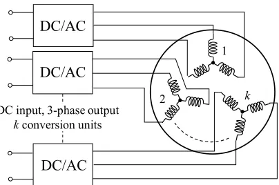
Fig. 1. Multiphase topology with multiple three-phase units.

In this configuration, each three-phase set is supplied by an independent three-phase inverter. The inverter units share the control algorithm only at high level to obtain full fault-tolerance. If a three-phase inverter unit goes in fault, it is disconnected from the DC power supply. The main advantage of this configuration is the use of the well-consolidated three-phase power electronics modules, reducing the converter size, cost and design time [11].

B. Machine Modeling

The mathematical description of the multi three-phase topology can be performed by using the Multi-Stator (MS) approach. Introduced in [12] and recently applied in [13] for a quadruple-three phase machine, it considers the stator as a multiple of phase set, while the rotor is seen as a three-phase structure [14].

This section presents a generic MS modeling approach for an Induction Machine (IM) with the hypothesis of sinusoidal winding distribution. The number of phases of the machine is

nph=3n and k=1,2,…,n is the index number of a single three-phase set. The stator parameters of the three-three-phase sets are considered different each other in order to deal with the most general case. For simplicity, the iron losses are neglected.

For each three-phase statork-set, the stator voltage equations are:



sabck



sk



sabck

 

sabck



dt d i

R

v _,   _,   _, (1)

where:



x_sabc,k







x_sak x_sbk x_sck



tis a stator vector defined for the three-phase set (abc)kand defined in own stator

coordinates;

sk

R is the stator resistance for the three-phase setk. Assuming a rotor cage that is equivalent to a three-phase wound rotor, the rotor voltage equations are:



rabc



r

 

rabc



rabc



dt d i R

v [0]    (2)

where:



x_rabc

 

 x_ra x_rb x_rc



tis a rotor vector in rotor phase coordinates;

r

[image:2.595.341.525.54.189.2]

R is the rotor resistance.

Fig. 2. Equivalent circuit of IM in stationary (α,β) frame. The IM magnetic model is described by (3) and (4):























sk r

  

rabc

n

z

z sabc sz sk k

sabc lsk k

sabc L i  M i  M i

 _

 



1

, ,

, (3)





 















r r

  

rabc

n

z

z sabc sz r rabc

lr

rabc L i  M i  M i

 _

 



1

, (4)

where:



M_sksz



is a 33 mutual inductance matrix between two stator windings;



Mskr



is a 33 mutual inductance matrix between the

stator windings ofkset and the rotor;



Mrsz



is a 33 mutual inductance matrix between the

rotor and the stator windings ofzset;



Mrr



is a 33 mutual rotor inductance matrix; lsk

L is the stator leakage inductance for the three-phase setk;

lr

L is the rotor leakage inductance.

All rotor parameters from (2-4) are referred to the stator. The MS approach needs the application of the general Clarke transformation to get the machine model in stationary (,β)

frame:

 

 

 

















     

   

   

  

   

  

 

2 1 2

1 2

1

3 2 sin 3 2 sin sin

3 2 cos 3 2 cos cos

3 2

k k

k

k k

k

k

T (5)

where k is the angle considered for a three-phase k-set; this

angle is defined as the position of the first phase (a-phase) of the

k-set with respect to the-axis. By applying (5) to (1)-(4), the stator model for IM in (,β) reference frame becomes:

 

   ,   ,

, sk sk sk

sk R i _dtd

v (6)

The rotor equations are transformed into stator stationary reference frame using (5) with k = r, where ris the rotor

electrical position:

 

    



 _{, , ,}

0 _{r r r} j _{r r}

dt d i

R (7)

where ωris the rotor electrical speed. 1

2 k

DC/AC

DC/AC

DC/AC

DC input, 3-phase output

kconversion units

sn

R Llsn Llr

m

L Rr



    r r, j 

, 1

s

v

 ,

sn

v

 ,

sn

i

() frame

 , 2

s

i

 , 1

s

i

 , 2

s

v

1

s

R

2

s

R Lls2 1

ls

L



 ,

r

The IM magnetic model in stationary frame is obtained as:           



_, 1 , ,

, m r

n z sz m sk lsk

sk L i L i L i (8)

           



_, 1 , ,

, m r

n z sz m r lr

r L i L i L i (9)

where L_m is the magnetizing inductance.

The IM electromagnetic torque is given by (10) and represents the sum ofnouter (vector) products:







       n z sz sz i p T 1 , , 2 3 (10)

According to (6)-(10), the MS approach definesndifferent stator flux linkage vectors and current vectors and the total electromagnetic torque is the sum of the contributions of then

stator sets that interact with the three-phase rotor. Therefore, the equivalent circuit of the IM corresponding to the MS modeling approach is shown in Fig. 2.

The stator and rotor equations can be referred to a generic rotating reference frame (d,q) at speede. Indeed, by applying

the conventional rotational transformation, the (d,q) voltage equations become: dq sk e dq sk dq sk sk dq

sk R i _dtd j

v _,   _,   _,    _, (11)



e r



rdq dq

r dq r

r _dt j

d i

R _{, , ,}

0         (12)

The IM magnetic model in rotating (d,q) frame is formally identical with (8-9), with the difference that all vectors (fluxes and currents) are referred to the (d,q) frame instead of the (,β)

stationary reference frame.

III. MODELPREDICTIVEFORMULATION

The implementation of a predictive system requires first the computation of the machine’s state equations and subsequently a good method to discretize them. This procedure is well consolidated for phase machines but not for multi three-phase configurations having a higher number of active state variables.

A. Machines’s State Equations

The proposed model predictive algorithm uses a DFVC scheme based on the MS-approach [13-16]. Consequently, the stator currents and the stator fluxes must be considered as main state variables. It is necessary to introduce the following preliminary variables:

lr m

m

r _{L L}

L k   , lsk m m

sk _L L_L

k   , r lr m r _R L L    (13)



     n k z z lsz z lr r

k k L _Lx

c 1 , lsz z lr r

z k L _Lx

c    (14)

where ݔ௭ is a logic value depending by the state of the

consideredz-set (0 off, 1 on). In this way, it is possible to adapt the equations of the remained active sets after open-windings fault events.

The state equations with the MS approach for a single k

three-phase set (k=1…n) leads to:

k dq sk k v dq sk eq dq sk k eq dq sk k

eq _dt Z i f k v C

i d

L  ,  _,  _,   _,  _,  _, 

, (15) dq sk e dq sk dq sk sk dq

sk R i v j

dt d , , , ,        (16)



  _{     }     n z dq sz r r dq r slip r dq

r j R k i

dt d 1 , , 1

, ( ) (17)

where: Leq,k(1ck)Llsk krLlr

)

( _{, ,}

,k eqk eqk

eq R j X

Z   



k



sk sk

r r k

eq _k R c

k R

R _,    1

k eq slip lsk k r k

eq c L L

X ,      ,

r r

eq j

f  1  _,

k k

v c

k _, 1 ,_slip _e_r The term Ck contains the coupling terms between the

considered k-set with the other onesz=1…n, z≠k. This is the direct consequence of the application of MS-approach with respect to the conventional Vector Space Decomposition (VSD) [8,13]. The coupling termCkis computed as:



       n k z z dq sz z eq dq sz z

k c v Z i

C 1 , , , ) ( (18)

where: Z_eq,z R_eq,z jX_eq,z z sz r r z

eq R k R c

R ,     , Xeq,z rczLlsz

The equations (15)-(17) represent the complete electromagnetic dynamic model of a multi-three phase machines with a generic number of three-phase setsn. These equations are the starting point for the implementation of any model predictive control.

B. Discretization of the State Equations

The state equations (15)-(17) must be converted into their discrete time equivalents. This operation is not easy to perform, even for a three-phase case. In fact, it is necessary to compute the general relationships of the eigenvalues and related eigenvectors of a high order system. For this reason, in this work the Euler’s approximation is proposed.

Independently by the considered equation from the set (15)-(17), each of them has the same structure where from a side there is the derivative of the considered variable_ܺതwhile, on the other side, the forcing termsܨത:

) ( ) , (F t F t X

dt

d _

(19)

The Euler’s approximation of (19) in order to convert the time domain from continuous to discrete is:

where TS is the sample time for the discretization and τ the

generic sample time instant. As an example, the application of (20) to (16) leads to:



( ) ( ) ( ) ( )



...

... ) ( )

1 (

, ,

, ,

, ,

             

      

dq sk e dq

sk dq sk k s S

dq sk dq

sk

j v

i R

T (21)

Since this method is a first-order approximation of the real discrete equations, it is necessary to choose a proper value of sample time TS. Nevertheless, in an electric drive this value usually corresponds with the switching frequency of the power converter and therefore often predefined. Consequently, the accuracy of the Euler’s discretization will depend by the electric fundamental frequency together with a proper estimation of the machine’s parameter.

IV. MACHINECONTROLSCHEME

The application of a model predictive algorithm does not depend on the choice of the control type. In fact, MPC allows at improving the performance of already predefined control scheme by replacing the traditional PI controller with a better selection of the voltage references.

The proposed model predictive algorithm uses a DFVC scheme based on the MS-approach. The DFVC combines the advantages of a direct flux regulation (as for constant frequency direct torque control) with current regulation (as for vector control) [13,15,16]. The main advantage of the MS-approach is the possibility to build a modular machine control where each three-phase set is independently controlled. In this way, post open-winding fault operations or torque sharing operations become easy to perform.

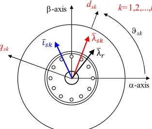
According to the torque demand and the operating speed, the MS-based DFVC aims to controllingnstator flux vectors inn

[image:4.595.352.509.59.192.2]

overlapped stator flux frames (dsk,qsk,k=1,2,…,n), as shown in

Fig. 3.

A. Stator Flux and Torque Equations

The machine model in multiple stator flux reference frames (dsk,qsk, k=1,2,…,n) is described by the equations (15)-(17),

where the synchronous speed e corresponds with the

pulsation/speed of the considered stator flux vector. In theory, this value must be defined set by set. However, since the machine control aims to setnoverlapped stator flux frames, the differences between the three-phase sets can be neglected.

Relevant attention must be given to the stator flux and torque (10),(16) equations. In fact, the DFVC is implemented in rotating stator flux frame and this leads to important simplifications.

In terms of stator flux vectors, each of them is aligned in the owndsk-axis and so all fluxqsk-axis components are zero:

ds sk ds sk sk

sk _{R i v}

dt d

, ,     

(22)

while in terms of total electromagnetic torque:





    

n

k

qs sk sk i p

T

1

, )

( 2

[image:4.595.308.558.218.357.2]

3 ₍₂₃₎

Fig. 3. Multiple direct flux vector control based on MS-approach.

Fig. 4. Stator flux observer.

The model (22),(23) leads to the following considerations:  Thedsk– axis voltage (vsk,ds) directly imposes the

stator flux magnitude λsk,k=1,2..,n.

 The torque contribution of one stator winding setk

is controlled by regulating the correspondingqsk–

axis current (isk,qs), using the voltage component

vsk,qs,k=1,2..,n.

B. Stator Flux Observer

The flux observer is shown in Fig. 4. The flux observer estimatesnstator flux vectors_sk,k=1,2,…,n, corresponding to thenstator three-phase sets. The flux observer is based on the back-EMF integration at high speed and on the rotor magnetic model at low speed [17].

At low speed, the stator flux vectors are computed from the rotor flux using (7)-(9). The rotor model is sensitive with the rotor time constantr, but this affects only the machine starting.

At high speed, the flux estimates depend only on the stator resistances Rsk. The detuning on this parameter has very low

effects on the flux estimation, so the flux observer is very robust against parameters detuning.

To improve the performance at low speed, a dead-time (DT) compensation scheme has been implemented for each stator set using the solution described in [18].

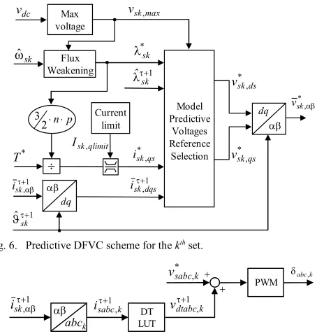
C. Predictive Direct Flux Vector Control (DFVC) scheme

The proposed predictive DFVC scheme contains n

independent modules that are separately implemented in the overlapped stator flux frames (dsk,qsk,k=1,2,…,n), as shown in

Fig. 6.

-axis -axis dsk

ଓҧ௦௞ λത௦௞

qsk

λ ത_௥

sk

k=1,2,...,n

sk

Rˆ



k

g

 ,

sk

v  ,

dtk

v



ˆsk,



 ,

~ sk

  

 

u u 

sk ˆ

sk ˆ

sk ˆ

 ,

sk

i

n k1,2,..,

1 

r

ˆ



dq_

m 

dqm r,

 r,

λ௥

→

λ௦௞









 dq 

, 1

s

i

 , 2

s

i

 ,

sn

i

 is,dqm

m Lˆ



1,

~ s



2,

~ s



 ,

Fig. 5. Predictive direct flux vector control control scheme of a generic multi three-phase machine.

A single DFVC module is operated as for a three-phase machine and does not interact with the other modules.

The reference flux is generated by a Flux-Weakening (FW) block that imposes the rated flux (corresponding to one statork -set) below the base speed and a flux that depends on the available DC link inverter voltage and the synchronous speede

at flux-weakening. The torque-producing component in stator flux frame is computed for each stator setkas:



sk



qs

sk T n p

i*  * 3₂  ˆ

, ,k=1,2,…,n (24)

The torque producing components for then stator sets are further limited according to the machine maximum current. The flux computation at flux weakening is implemented as in [15]. The independent flux-current control of the stator sets keeps balanced their currents and allows the operation with one or more stator sets turned off in case of faults.

With respect to a conventional DFVC based on the MS approach [13,16], the application of a predictive algorithm requires additional blocks, as shown in Fig. 5. The first one is the Model Predictive Estimator (MPE) where is performed the prediction of the variable of interest for the next sample time

instant (τ+1). In the MPE block are implemented the state

equations (15)-(17) with the application of the Euler’s discretization (20). The prediction of the variables is performed

in the stationary frame (α,β) in order to use the estimates of the

stator flux observer directly. Therefore, the equations (15)-(17) are implemented by setting the synchronous speedeto zero.

The MPE presents a modular structure in order to preserve the control scheme modularity. In fact, it is structured in n

predictive estimators where each of them performs the predictive estimation for the dedicatedk-set.

From the MPE, the values of stator fluxes and stator currents

for the next sample time instant (τ+1) are obtained. From the

predicted values of the stator currents it is possible to estimate the Dead Time (DT) errors of the power converter for the next

sample time instant (τ+1). In this way, it is possible to apply an

[image:5.595.315.542.54.294.2]

accurate feed-forward compensation, as shown in Fig. 7. This action leads to relevant improvements in the currents waveforms, especially at low speed and no load-condition.

Fig. 6. Predictive DFVC scheme for thekth_set.

Fig. 7. Predictive Dead Time (DT) errors compensation for thekth_set. For eachk-set, the position of the stator flux vectorˆsk1, for the next sample time instant (τ+1), is computed. This is

necessary to perform the rotational transformation in order to obtain the (dsk,qsk) current values i_sk_,1_dqs for the next sample time instant (τ+1). The prediction of the angle ˆsk1is also necessary

to perform the rotational transformation for the computation of

the next sample time (τ+1) output reference voltages vsk*,. The predicted value of currents i_sk_,1_dqs and stator flux amplitude ˆsk1, together with the references of stator flux

amplitude *

sk

 and qsk-axis current isk*,qs, are used for the

computation of the voltage references vsk*,, as shown in Fig. 6.

D. Predictive Reference Voltages Selection

The proposed model predictive algorithm uses the machine inverse model for the control of the reference variables. Practically, the voltages reference applied at the next sample

time instant (τ+1) establish the evolution of the state variables at the next step (τ+2):

) 1 ( )

1 ( ) 2

( X  T F 

X _S (25)

From (25), to set the value of the generic state variableܺതto a target valueܺത∗_{it is necessary to satisfy the (26):}

S T

X X

F*(_1)_ * (1) ₍₂₆₎

Referring to the equations (15)-(17), the application of the (26) corresponds to invert the machine model in order to obtain the voltage references. The proposed method for the computation of the voltages reference is shown in Fig. 8.

n sabc

i ,1

DT

 , 1n s

i

 , 1n dt v

Direct Clarke

Stator flux observer

Speed computation

m

 m

Voltage Reconstruction

PWM

n

abc

 ,1 dc

v

 , 1n s

v

* , 1n

s

v *

1 , n sabc

v 

Inverse Clarke

Model Predictive

Estimator ˆs1_n,_ Model

Predictive DFVC *

T

max

I

1 1

ˆ 

s n 1

, 1

  n s

i 1

1

ˆ 

s n

n

s

ˆ1

3 3

3

IM 3n-ph

dc v

 

n

s

ˆ1

 , 1n s

v

 , 1n s

i

 , 1n dt

v

Max voltage

Flux Weakening

*

sk



1

ˆ

sk max sk

v _,

dc

v

Current limit

sk

ˆ

*

T skqlimit

I ,

* ,ds sk

v

* ,qs sk

i 

p n  2 3



dq

1

ˆ

sk 1 ,  



sk

i isk,1dqs



dq *

,

sk

v

* ,qs sk

v Model Predictive

Voltages Reference

Selection

1 ,

 

 sk

i _

k

abc

1 ,

 

k sabc

i _DT

LUT

1 ,

 

k dtabc

v

  *

,k sabc

v

PWM abc,k

[image:5.595.38.289.54.212.2]

[image:6.595.356.523.58.203.2]

Fig. 8. Voltages reference computation for thekth_set.

1) Voltage reference computation on dsk-axis

By considering the (22), the computation of thedsk– axis

voltage reference is performed as:

S sk sk ds sk sk ds

sk R i _T

v*_,   _,1 * ˆ1 (27) The dsk – axis voltage reference, together with the inverter

voltage limit define the limits of theqsk– axis component, as

the conventional DFVC scheme.

2) Voltage reference computation on qsk-axis

With respect to thedsk– axis component, the computation of

the qsk– axis reference voltage must be performed in two steps.

In fact, the qsk– axis current equations (15) contains the voltage

coupling between the sets. Therefore, first is necessary to compute the linear combinations of voltages reference as function of the qsk– axis current references:



      n k z z qs k qs sz z qs sk k

v v c v F

k 1 * , * , * , , (28) where:                                



kcomp

n k z z ds sz z eq qs sz z eq sk r ds sk k eq qs sk k eq qs sk qs sk S k eq qs k K i X i R i X i R i i T L F , 1 1 , , 1 , , 1 1 , , 1 , , 1 , * , , * , ) ( ˆ ... ... ) ( (29)

In (29) there is a new term called Kk,comp. It represents the

output of an integral regulator. It is computed as:

) (*_{, ,} , 1 , ,    _{    } qs sk qs sk k i S comp k comp

k K T k i i

K (30)

Practically, the (30) represents the integral regulation of the

qsk– axis current in a traditional DFVC scheme. Nevertheless,

the purpose of this compensation is completely different. In fact, the predictive computation of the variables loses its accuracy at high frequency/speed, caused by the approximation of the Euler’s discretization. Furthermore, the predictive algorithm is based on the machine’s parameters and consequently is influenced by the estimation errors. These problems cause torque permanent error, especially due by the inaccuracy in the

qsk– axis.

[image:6.595.50.272.61.198.2]

Fig. 9. Asymmetrical 6-phase induction machine configuration (2x3ph). TABLE I. CHARACTERISTICS OF THE MACHINE

Main Data

Number of phases 6 (2x3-phase, star connected) Rated phase voltage 230 Vrms

Generating mode

Continuous output power 10 kVA Constant power range 6000 to 15000 rpm

Overload 150% 5 min

Cooling system forced air ventilation

Through the application of the integral regulation (30), the torque error converges to zero with a dynamic related the value of the integral gainki,k and the voltage margin of the integral

compensator (a good compromise is 5%-10% of the total phase voltage margin). The design of this regulator is not critical. It does not influence the dynamic behavior of the drive but only the steady-state operations.

From the (28) it is necessary to extrapolate the qsk – axis

voltage reference v*_sk,qs. Therefore, it is necessary to apply the following decoupling operations:

                                                     * , * , 2 * , 1 , 2 1 2 1 2 , 1 2 1 , * , * , 2 * , 1 ... ... ... ... ... ... qs n qs qs n v n n v n v qs sn qs s qs s F F F k c c c c c c k c c c k inv v v v (31)

The application of (31) is not critical. In fact, the analytical solutions can be computed offline. In the drive, it is sufficient to implement the analytical results. These are valid also in case of open-winding fault events being the coefficient of matrix defined as (14).

V. EXPERIMENTALRESULTS

The performance of the proposed control has been validated with an asymmetrical six-phase induction machine using a double-three-phase stator winding configuration. The main features of the machine are shown in Table I [16]. The stator has 6 phases with two slot/pole/phase, forming a double-three-phase winding with relative shift of 30 electrical degrees among the two three-phase sets (akbkck),k=1,2, as shown in Fig. 9.

n z1,2,..., *

sk



1

ˆ sk Inverse Flux Model max sk v _, * ,ds sk v 1

u u2

Inverse q-Current Model * ,qs sk i 1 ,   qs sk i q-axis Voltage Decoupling * ,qs k F * ,qs z F k z * ,qs sk v n k1,2,...,

ݑଵ ଶ− ݑଶ ଶ a1 a2 b1 c1 b2 c2

a2-axis

c1-axis

c2-axis

b2-axis

b1-axis

-axis

-axis

[image:6.595.316.544.235.352.2]

[image:7.595.63.277.52.158.2] [image:7.595.325.549.65.261.2]

Fig. 10. Machine under test (right) and the driving machine (left)

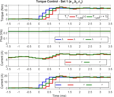
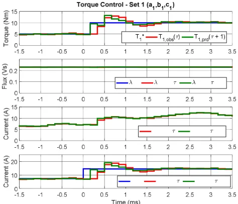
Fig. 11. Fast torque transient from no-load up to 150% rated torque (24Nm) at -6000 rpm, Set 1. From to to bottom: reference torque, observed torque and predicted torque (Nm); reference stator flux, observed stator flux and predicted stator flux; observedds1-axis current and predictedds1-axis current; reference

qs1-axis current, observedqs1-axis current and predictedqs1-axis current. The machine has been mounted on a test rig for development purposes. The shaft of the machine prototype is connected with a driving machine (Fig. 10). The power converter consists of two independents three-phase inverter IGBT power modules fed by a single DC power source of 550V. All inverter units are based on the Infineon 100A/1200V, MIPAQ three-phase IGBT power module. The digital controller is the dSpace DS1103 development board that uses a dedicated FPGA-based interface to communicate with the inverter modules through optical fibers. The sampling frequency and the inverters switching frequency have been set at 6 kHz.

A. Healthy operation

[image:7.595.46.284.183.386.2]

The machine has been tested in generation mode with a negative speed of -6000 rpm imposed by the prime mover (speed controlled), while the machine is torque controlled. The generator operation in healthy conditions is shown in Figs. 11-13 for fast torque transient (40Nm/ms) from zero up to 24 Nm (0 to 15kW mech., 150% of the rated value). It can be noted how the two three-phase sets are perfectly balanced with a fair distribution of the total power (12Nm - 7.5kW mech. for each set), as can be seen in Fig. 13. It can be noted the right prediction of torque, currents and stator fluxes, as shown in Figs. 11-12. Furthermore, the perfect torque response (as the well-known DBTFC).

Fig. 12. Fast torque transient from no-load up to 150% rated torque (24Nm) at -6000 rpm, Set 2. From to to bottom: reference torque, observed torque and predicted torque (Nm); reference stator flux, observed stator flux and predicted stator flux; observedds2-axis current and predictedds2-axis current; reference

qs2-axis current, observedqs2-axis current and predictedqs2-axis current.

Fig. 13. Fast torque transient from no-load up to 150% rated torque (24Nm) at -6000 rpm. Ch1:ia1(10A/div), Ch2:ia2(10A/div).

[image:7.595.310.558.325.495.2] [image:7.595.309.558.521.695.2]

[image:8.595.45.282.54.257.2]

Fig. 15. Inverter 2 shut off during generation mode at -6000rpm and 10Nm. Set 1. From to to bottom: reference torque, observed torque and predicted torque (Nm); reference stator flux, observed stator flux and predicted stator flux; observed ds1-axis current and predicted ds1-axis current; reference qs1-axis current, observedqs1-axis current and predictedqs1-axis current.

B. Faulty operation

The drive “fault ride-through” capability when one inverter unit is suddenly disabled is shown in Figs. 14-16 (inverter 2 off), with fast and good dynamic. The healthy unit exhibits sinusoidal currents that increase in order to keep the same torque and machine flux, as shown in Fig. 14. This is the proof of the modularity of the MS-based control schemes, with the maximum degree of freedom in the control of the single three-phase sets.

VI. CONCLUSIONS

The paper proposes a model predictive control (MPC) for multiphase induction machine configured as multiple three-phase structures. The predictive algorithm is implemented on the basic structure of the Direct Flux Vector Control (DFVC) scheme for simultaneous flux and torque control. The performance of the proposed control has been validated with a double-three-phase induction machine. The experimental results demonstrate the feasibility of the proposed drive solution both in healthy and faulty operations (open-winding fault events).

REFERENCES

[1] P. Correa, M. Pacas, J. Rodrìguez, “Predictive Torque Control for Inverter-Fed Induction Machines”,IEEE Trans. Ind. Electron., vol. 54, no. 2, 2007, pp. 1073-1079.

[2] M.Preindl, S. Bolognani, “Model Predictive Direct Torque Control with Finite Control Set of PMSM Drive Systems, Part 1&2”,IEEE Trans. Ind. Informatics, vol. 9, no. 4 & no. 2, 2013, pp. 1912-1921 & pp. 648-657. [3] B. Boazzo, G. Pellegrino, “Predictive Direct Flux Vector Control of

Permanent Magnet Synchronous Motor Drives”, IEEE-ECCE,2013,pp. 2086-2093.

[4] Y. Zhang, H. Yang, “Model Predictive Torque Control of Induction Motor Drives With Optimal Duty Cycle Control”,IEEE Trans. Power Elect., vol. 29, no. 12, 2014, pp. 6593-6603.

[5] C. A. Rojas, J. Rodríguez, F. Villarroel, J. R. Espinoza, C. A. Silva, M. Trincado, “Predictive Torque and Flux Control Without Weighting Factors”,IEEE Trans. Ind. Elect., 2013, vol. 60, no. 2, pp. 681-590.

Fig. 16. Inverter 2 shut off during generation mode at -6000rpm and 10Nm. Set 2. From to to bottom: reference torque, observed torque and predicted torque (Nm); reference stator flux, observed stator flux and predicted stator flux; observed ds2-axis current and predicted ds2-axis current; reference qs2-axis current, observedqs2-axis current and predictedqs2-axis current.

[6] S. A. Odhano, A. Formentini, P. Zanchetta, R. Bojoi, A. Tenconi, “Finite Control Set and Modulated Predictive Flux and Current Control for Induction Motor Drives”, Conf. Rec. IEEE-IECON, 2016, pp. 2796-2801. [7] J. W. Kelly, E. G. Strangas, and J. M. Miller, “Multi-phase inverter

analysis”, Conf. Rec. IEEE-IEMDC, 2001, pp. 147–155.

[8] Y. Zhao and T.A. Lipo, “Space vector PWM control of dual three-phase induction machine using vector space decomposition”,IEEE Trans. Ind. Appl.., 1995, vol. 31, no. 5, pp. 1100-1108.

[9] F. Barrero, J. Prieto, E. Levi, R. Gregor, S. Toral, M.J. Duran, and M. Jones, “An Enhanced Predictive Current Control Method for Asymmetrical Six-Phase Motor Drives”, IEEE Trans. Ind. Electron.,2011, vol. 58, no. 8, pp. 3242-3252.

[10] Y. Wang, S. Tobayashi, and R.D. Lorenz, “A Low-Switching-Frequency Flux Observer and Torque Model of Deadbeat–Direct Torque and Flux Control on Induction Machine Drives”,IEEE Trans. Ind. Applicat., vol. 51, no. 3, 2015, pp. 2255-2267.

[11] W. Cao, B. Mecrow, G. Atkinson, J. Bennett, and D. Atkinson, “Overview of Electric Motor Technologies Used for More Electric Aircraft (MEA)”,

IEEE Trans. Ind. Electron., 2011, vol. 59, no. 9, pp. 3523-3531. [12] R.H. Nelson and P.C. Krause, “Induction machine analysis for arbitrary

displacement beween multiple winding sets",IEEE Trans. Power Appl. and Systems, vol. PAS-93, 1974, pp. 841-848.

[13] S. Rubino, R. Bojoi, A Cavagnino, and S. Vaschetto, “Asymmetrical Twelve-Phase Induction Starter/Generator for More Electric Engine in Aircraft”, Conf. Rec. IEEE-ECCE, 2016, pp. 1-8.

[14] R. Bojoi, S. Rubino, A. Tenconi, S. Vaschetto, “Multiphase electrical machines and drives: A viable solution for energy generation and transportation electrification“, EPE 2016, pp. 632 – 639.

[15] G. Pellegrino, R. Bojoi, and P. Guglielmi, “Unified Direct-Flux Vector Control for AC Motor Drives”,IEEE Trans. Ind. Appl., 2011, vol. 47, no. 5, pp. 2093-2102.

[16] R. Bojoi, A. Cavagnino, A. Tenconi and S. Vaschetto, “Control of Shaft-Line-Embedded Multiphase Starter/Generator for Aero-Engine”,IEEE Trans. Ind. Electron., vol. 63, no.1, 2016, pp.641-652.

[17] P.L. Jansen and R.D. Lorenz, “A Physically Insightful Approach to the Design and Accuracy Assessment of Flux Observers for Field Oriented Induction Machine Drives”,IEEE Trans. Ind. Appl., vol. 30, no.1, pp. 101-110, 1994.

[image:8.595.329.546.62.246.2]