APS/123-QED
Interpolation of intermolecular potentials using Gaussian processes.
Elena Uteva a, Richard S. Graham b, Richard D. Wilkinsonc and Richard J. Wheatleya.1 aSchool of Chemistry, University of Nottingham, Nottingham NG7 2RD,
UK.
bSchool of Mathematical Sciences, University of Nottingham, Nottingham NG7 2RD,
UK.
cSchool of Mathematics and Statistics, University of Sheffield, Sheffield, S10 2TN,
UK.
(Dated: 23 May 2017)
A procedure is proposed to produce intermolecular potential energy surfaces from
limited data. The procedure involves generation of geometrical configurations using
a Latin hypercube design, with a maximin criterion, based on inverse internuclear
distances. Gaussian processes are used to interpolate the data, using over-specified
inverse molecular distances as covariates, greatly improving the interpolation.
Sym-metric covariance functions are specified so that the interpolation surface obeys all
relevant symmetries, reducing prediction errors. The interpolation scheme can be
applied to many important molecular interactions with trivial modifications.
Re-sults are presented for three systems involving CO2, a system with a deep energy
minimum (HF−HF) and a system with 48 symmetries (CH4−N2). In each case the
procedure accurately predicts an independent test set. Training this method with
high-precision ab initioevaluations of the CO2−CO interaction enables a
parameter-free, first-principles prediction of the CO2−CO cross virial coefficient that agree very
well with experiments.
I. INTRODUCTION
This article concerns a central problem in molecular physics: quantitatively predicting
macroscopic material properties from first-principles molecular physics. There are numerous
practical applications to this problem, including the molecular design of materials,
manufac-ture and industrial processing. Such applications would be better understood and addressed
by exploiting predictions, from molecular first principles, of properties and processes such
as solubility, phase separation, osmosis, gas diffusion, crystallisation and nucleation.
Intermolecular potential energies can often be calculated accurately enough to be useful.
Thus the problem above can be solved, in principle, by computing molecular interactions
from ab initio quantum mechanics and macroscopic properties from statistical mechanics.
However, in practice, the computational cost of directly combining these two techniques
is hopelessly expensive in all but exceptional cases. The cost of evaluating the energy at
a single point is significant (often minutes or hours of time). Thus, it is necessary to fit
or interpolate calculated energy data at a limited number of points to produce a potential
energy surface.
In this article a machine-learning approach is applied to the problem. Machine-learning
algorithms have recently produced very rapid progress in computer mastery of complex
games, such as Go1, and they have enormous potential to surmount recalcitrant problems
in the physical sciences. The approach herein produces a flexible and widely applicable
algorithm to interpolate calculations of intermolecular potential energies, leading to a fast
method to compute the potential energy surface. The algorithm’s significant advantages
include high accuracy, the need for only comparatively small input data sets, and the
gen-erality to capture new molecular systems with little or no modification, leading to broad
applicability and significant savings in researcher time.
The efficacy of the method is shown by comparison with current best practice in
rep-resenting potential energy surfaces. Examples of careful, elaborate fits of calculated data
include the potential energy surface of CO2−Ne2, where a root mean square error (RMSE)
∼0.15 µEh was quoted (1Eh ≈27.211 eV≈2625.5 kJ mol−1); a RMSE of about 0.6 µEh in
the well region (energyE <0) of CO2−H23; and a maximum error of about 2% of the well
depth in the well region of CH4−N24. Fits with much larger errors are commonplace in the
indepen-dent data, a procedure which is prone to over-estimating predictive accuracy. Interpolations
of intermolecular potential data are less common. Cubic splines are the most popular
in-terpolation method, for example in work on CO2−Ar5. In contrast, Gaussian process (GP)
interpolation, of which cubic splines are a special case6,7, has been relatively little used8,9,
despite its promise in other applications. Applications include solid-state potentials10,11,
conformational energies12, and the difference between calculated intermolecular potentials
of water13. The accuracy and speed of GPs compared to other machine learning techniques
was demonstrated for the electronic polarisation of water clusters14. The same group later
applied GPs to the atomic multipole moment surface of ethanol15, the electrostatic
interac-tion energy between Na+and water molecules16and the electrostatic energy of cholesterol17.
It is demonstrated here that with a small set of training points and a carefully chosen
coor-dinate system, a general symmetric Gaussian process interpolation scheme can achieve high
predictive accuracy and that the resulting PES can accurately predict experimental data.
II. GAUSSIAN PROCESS MODELLING
The approach involves two sets of data. A set of training data (between 20-1000 points)
is used to train the model, and a larger set of grid data is used to test the model’s predictive
performance. Both datasets are described below. No knowledge of the test data is used
during training.
Data sets of the intermolecular interaction energy of the bimolecular complexes CO2−Ne,
CO2−H2, CO2−CO, HF−HF and CH4−N2 are calculated as a function of their
configu-rational geometry. These complexes are chosen to cover a range of intermolecular bond
strengths and symmetries, and to be small enough that an extensive set of data can be
pro-duced for testing the interpolations. For the same reason, all molecules are approximated as
linear rigid rotors in their vibrational ground state, with fixed bond lengths, although the
interpolation method can be extended straightforwardly to non-rigid molecules. Energy
cal-culations are carried out in Molpro18 using second-order Møller-Plesset perturbation theory
(MP2) and augmented correlation-consistent triple-zeta (aug-cc-pVTZ) basis sets. Basis set
superposition errors are corrected using the full counterpoise correction procedure.
Jacobi coordinates are used to describe the multi-dimensional potential energy
CO2−Ne, θ is the angle between r and the CO2 axis. For CO2−H2,θ1 is the angle between
r and the CO2 axis, θ2 is the angle between r and the H2 axis, and φ is the torsional angle
of the H2 axis. Analogous coordinates are used for HF−HF and for CO2−CO, whereθ2 = 0
corresponds to the O from the CO molecule being closest to the CO2. For CH4−N2, the
N2 molecule is placed at a position relative to the C of CH4 at position (r, θ, φ) in polar
coordinates, and the N-N axis is rotated to orientation (α, β), also in polar coordinates.
The C-O (for CO2), C-O (for CO), H-H, H-F, C-H and N-N bond lengths are taken to be
1.1632 ˚A, 1.128 ˚A, 0.77 ˚A, 0.92 ˚A, 1.09 ˚A and 1.098 ˚A, respectively. An energy cutoff of
Ecut = 0.005 Eh is imposed (0.02 Eh for HF-HF due to its much larger well depth), and
configurations with intermolecular potentials above this cutoff are excluded from the data
sets. Configurations are also excluded if any interatomic distance is below 1.5 ˚A or if all
interatomic distances are above 8.5 ˚A. Separations below this would also be excluded by the
energy cutoff, but this criterion saves time that would be spent in calculating unhelpfully
large energies, and beyond 8.5 ˚A it is more efficient to use an asymptotic expansion of the
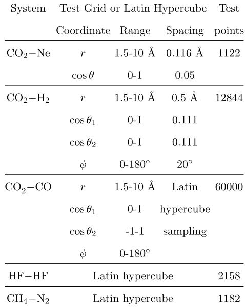
energy, as discussed later. Details of the test data used for model assessment are given in
Table I.
Gaussian processes (GPs) are used extensively in machine learning and statistics as
re-gression models. The book of Rasmussen and Williams7 contains a detailed introduction
to GPs, including several different but equivalent ways of understanding GPs. Like neural
networks (NNs), GPs are non-parametric models which have proved successful in creating
theory-free models of complex datasets. The advantage of GPs over NNs is that they are
mathematically tractable and interpretable, and allow prior information to be built in to
the model (such as symmetry, differentiability, and conditioning on derivative information).
The prior specification of a GP consists of a mean function (often taken as zero) and a
covariance function k(x,x0), expressing the covariance between f(x) and f(x0), where f is
the function being interpolated. Training data, consisting of observations of the value of f
at various locations, update the mean and covariance functions to give a posterior model
which predicts the function at any location.
Properties of the GP model are inherited from the covariance function, for example,
differentiability, continuity and stationarity. The intermolecular energy is a non-stationary
function of distance, as it varies rapidly at small interatomic separations, but more gently
TABLE I. Coordinates for the test (grid or LHC) data for each system. System Test Grid or Latin Hypercube Test
Coordinate Range Spacing points CO2−Ne r 1.5-10 ˚A 0.116 ˚A 1122
cosθ 0-1 0.05
CO2−H2 r 1.5-10 ˚A 0.5 ˚A 12844
cosθ1 0-1 0.111
cosθ2 0-1 0.111 φ 0-180◦ 20◦
CO2−CO r 1.5-10 ˚A Latin 60000 cosθ1 0-1 hypercube
cosθ2 -1-1 sampling φ 0-180◦
HF−HF Latin hypercube 2158
CH4−N2 Latin hypercube 1182
in practice it can be challenging to find a flexible form with the correct non-stationary
behaviour. It is simpler to transform either the inputs or outputs to achieve approximate
stationarity, which is addressed here by using the inverse interatomic distances as covariates
in the GP. Thus the GP coordinates are x = (1/r1, ...,1/rND) where ri is the interatomic
distance, running over all pairs of nuclei on different molecules. This results in an
over-specified system, for example with ND = 6 dimensions for CO2−H2. It is shown later that
this change in variables leads to a dramatic improvement in performance.
The training data should ideally cover evenly a single symmetry-distinct sub-region of
x space, and respect the geometric constraint. The general strategy is to generate many
candidate data sets (coordinates only, not energies), exclude points outside the symmetric
and geometric constraints, and select the candidate data set with the best distribution of
points. The placement of candidate data sets is based on Latin hypercube (LHC) sampling,
as explained in appendix B. Specifically, for CO2−Ne, CO2−H2 and CO2−CO, candidate
Table I. For HF−HF, three LHCs are generated and combined into one dataset: one uses
the F-F distance as the radial coordinate r, and keeps only those data points within the
LHC for which the F-F distance is the shortest of the four internuclear distances; the other
two LHCs are generated in the same way but with F-F replaced by H-H and H-F in turn.
The LHC for CH4−N2 is generated based on an H-N distance as the radial coordinate,
and uses only the data points for which the same H-N distance is the shortest of the ten
internuclear distances. For all cases, after generating the LHCs, deleting data points based
on the symmetric and geometric constraints, and combining the sets of points into one (for
HF-HF), the minimum separation of the remaining points is calculated in x space. The
candidate data set with the largest minimum separation is used as the training set. This
‘maximin’ approach aims to cover evenly the relevant region of xspace. See appendix B for
further details of this algorithm.
The Gaussian process has a zero mean function and a squared-exponential covariance
function
κ(x,x0) =σf2
ND
Y
i=1 exp
−(xi−x
0 i)2
2l2
i
(1)
where σf2 is the signal variance and li is the correlation length for each dimension. This
results in a stationary and infinitely differentiable model, called the ‘non-symmetric model’.
Here, symmetric refers to the permutations the interatomic distances under which the PES
should be invariant, because of molecular symmetries (see appendix C for further details).
In the non-symmetric model neither the kernel (covariance function) nor the training data
have these symmetries. Introduced later is a model in which the kernel has the appropriate
symmetries.
The potential energy surfaces obey various symmetries in x space. For example, for
CO2−Ne, the energy is invariant under the interchange of the two coordinates corresponding
to distances between Ne and each of the O atoms. Let G represent the permutation group
containing permutations of elements of x under which the energy surface is unchanged. If
it is assumed thatli =lj when coordinates xi and xj swap for some permutation inG, then
a covariance function of the form
ksym(x,x0) =
X
g∈G
κ(gx,x0). (2)
‘symmetric model’ based on this covariance function gives predictions that respect the
relevant symmetries, and usually significantly improves the performance, even within the
symmetry-distinct region covered by the test data, as shown below.
Results are obtained using the GPy package19, modified to include symmetric
covari-ance functions. Zero-mean Gaussian observation error7 is assumed on the function outputs
(referred to as a nugget in geostatistics), with standard deviation σn. Thus the model’s
hyperparameters are σf, σn and {li}. These hyperparameters are estimated by optimising
the log-likelihood over≈30 random restarts, which typically is sufficient to find the optimal
values multiple times.
The choice of inverse internuclear distances to transform to stationarity is important.
To illustrate this a ‘basic model’ GP is created, which uses internuclear distances r as
coordinates rather than 1/r, but is otherwise identical to the non-symmetric GP above,
having the same test and training data and a covariance function of the same form as
equation (1).
III. RESULTS
Predictive performance is measured using the root mean square error (RMSE) of the
GP predictions of the test data. Since the test data extensively cover the potential energy
surface, the RMSE is a reasonable guide to the expected ‘accuracy’ of the interpolation.
The methodology used here represents a demanding test of accuracy, since the GP has no
advance knowledge of the test data, only the far more limited training data, and equal
weighting is used for all test data, including positive interaction energies up to the potential
energy cutoff.
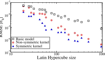
The results for CO2−Ne are shown in Figure 1. Models based on inverse intermolecular
distances dramatically outperform the basic model, being typically 2-3 orders of magnitude
more accurate for a given LHC size. Furthermore, even though CO2−Ne has only one
symmetry, the symmetric model is typically twice as accurate as the non-symmetric model.
Figure 2 shows similar results for CO2−H2. Here, the inverse distance models again strongly
outperform the basic model, achieving RMSEs < 10−6 E
h for a reasonable number of
training points. The symmetric kernel typically gives a factor of 2-10 improvement, with
10 100 1000
Latin Hypercube size
[image:8.612.214.395.70.176.2]10-8 10-7 10-6 10-5 10-4 10-3 RMSE [E h ] Basic model Non-symmetric kernel Symmetric kernel
FIG. 1. RMSE against LHC size for CO2−Ne. The lowest energy in the grid data is −2.90× 10⁻⁴ Eh.
of symmetries.
10 100 1000
Latin Hypercube size
10-7 10-6 10-5 10-4 10-3 RMSE [E h ] Basic model Non-symmetric kernel Symmetric kernel
FIG. 2. RMSE against LHC size for CO2−H2. The lowest energy in the grid data is−8.25×10⁻⁴E
h.
For HF−HF, the minimum energy in the test data is−6.17×10⁻³ E
h, which is about an
order of magnitude larger than for the other interactions. Probably as a consequence of this,
it is necessary to include training points up to at least 10−2 Eh, otherwise the prediction
of points on the repulsive wall is poor. Using a cutoff of 2×10⁻² E
h gives an RMSE of
1.6×10⁻⁴ Ehfor a symmetric GP with 59 training points, and the RMSE generally decreases
with increasing numbers of training points, to 1.8×10⁻⁵ E
h for 327 training points. The
RMSE in the negative-energy region is about 5×10⁻⁶ E
h for the latter GP; one or two
high-energy points dominate the overall RMSE. The inclusion of symmetry in the GP has
little effect on the RMSE for this interaction.
For CH4−N2, all 48 symmetry elements are included in the GP. Consideration of
symme-try is important for this interaction, even though all the training and test data are confined
within a single symmetry-distinct region of space. The minimum energy in the test data is
−6.98×10⁻⁴ Eh. With a training set of 106 points, the RMSE is 51×10−6 Eh for the
non-symmetric GP and 6.8×10⁻⁶ E
[image:8.612.216.394.285.387.2]these to 17×10−6 E
h and 1.3×10⁻⁶ Eh respectively.
For CO2−CO, with the symmetric GP, the RMSE is 6.7 ×10⁻⁵ Eh for 132 training
points, reducing to 1.1×10⁻⁵ E
h for 345 training points. The RMSE resulting from the
non-symmetric GP is generally a factor of ∼ 2 larger. Generating CO2−CO training data
by replacing LHC sampling of 1/r with 1/r2 improves performance, leading to RMSEs of
2.4×10⁻⁵ and 3.0×10⁻⁶ for 135 and 366 training points respectively, with the RMSEs
computed using the same test set as the above results.
2 3 4 Separation, r [Å] 0
0.1
Interaction potential [E
h
]
a) 4 Separation, r [Å]5 6 7 8 9
-1 0 1
Interaction potential [10
-4 E
h
]
Gaussian Process (241 point LHC) MP2 energies (below E
cut)
MP2 energies (above Ecut) Asymptotic expansion Repulsive cross-over
b) 6 8 10 12
Separation, r [Å]
-1 0
Interaction potential [10
-4 E
h
]
[image:9.612.179.431.228.333.2]c)
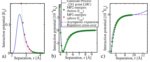
FIG. 3. CO2−Ne Molpro calculations and the GP model, at cosθ = 1 (linear geometry), in the repulsive (a), attractive (b) and long-range (c) regions. The long-range asymptotic expansion is
E =−(0.570 + 0.182 cos2θ)r−6−(1.704 + 7.266 cos2θ+ 1.785 cos4θ)r−8.
The performance of the GP outside the training region (E >0.005Eh and r > 8.5˚A) is
shown for CO2−Ne in Figure 3; results for other geometries and interactions are
qualita-tively similar. The extrapolation errors for short-range geometries satisfying the geometric
constraint, but withE > Ecut, are mostly a few percent or less. Even though the maximum
energy in the training set is limited to 0.005 Eh, the predicted repulsive wall continues up
to about 0.1 Eh. However, for small values of r the GP returns to its mean value of zero.
This unphysical behaviour can be corrected by crossing over to a strongly repulsive function
outside the geometric constraint. One example of the many possible choices is plotted in
Figure 3(a), namely
E =Emax 1
N
N X
i=1
(xi/xmax)12, (3)
where Emax is an estimate of the typical energy at the small-r edge of the geometric
constraint20 and x
max is the maximum inverse distance allowed by the geometric constraint
(0.67 ˚A−1 in this case). For large separations the GP tends to a small, but non-zero
the long-range asymptotic expansion obtained from a truncated multipole expansion of the
interaction energy (to second order) from intermolecular perturbation theory. Figure 3(c)
shows that smooth interpolation between the GP and this function will be straightforward.
IV. THE CO2−CO POTENTIAL ENERGY SURFACE AND SECOND
VIRIAL COEFFICIENT
Using the LHC training set for CO2−CO, based on sampling of 1/r2 and containing 135
training points, higher quality evaluations of the potential energy were produced for each
configuration. This involved complete basis set (CBS) extrapolation of the
counterpoise-corrected CCSD(T) interaction energy from the aVQZ and aVTZ basis sets. Training a
GP to this set gave a PES designed to be valid within the geometric constraint for energies
<0.005Eh. For large separations outside the geometric constraint, an asymptotic expression
consisting of atomic charges, dipoles, quadrupoles, static polarizabilities and C6 dispersion
coefficients is used instead of the GP. For separations smaller than the geometric constraint
the PES uses equation (3) with xmax = 0.5/A and˚ Emax = 0.456 Eh, which is the largest
energy in the LHC training data before applying the energy cut off. The code for this
potential energy surface is available in the Supplementary Material.
3 4 5 6 7 8 9 10
Separation, r [Å] -0.002
-0.001 0 0.001 0.002 0.003 0.004 0.005
Interaction potential [E
h
]
C-bonded isomer
[image:10.612.222.388.452.574.2]O-bonded isomer (shifted down by 0.001Eh)
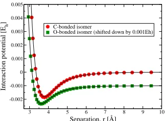
FIG. 4. Comparison of calculated interaction energies (symbols) with the GP-based PES (lines) for CO2−CO in the T-shaped configuration (θ1 =π/2) for the C-bonded (θ2 =π) and O-bonded
(θ2 = 0) isomers:. The C-bonded isomer includes the minimum energy.
The minimum energy for this PES, computed by numerical minimisation, is −1.827×
10−3Eh, which occurs at r = 3.791 ˚A, θ1 = π/2 and θ2 = π, corresponding to a T-shaped
experimental21 and theoretical22 work in which this C-bonded isomer was confirmed to be
the most stable. The C-C distance of 3.23 ˚A from the PES is 0.01 ˚A larger than the minimum
distance taken from the best literature calculation22; both are lower than the experimental
distance of 3.277 ˚A21, mainly as a result of non-rigidity of the intermolecular bond. A direct
calculation of the interaction energy for this geometry gives −1.859 ×10⁻³ E
h, which is
within 0.01×10⁻³ E
h of the best calculated value22. The difference of ∼ 0.03×10⁻³Eh
between the PES and calculation is similar to the RMSE of 0.024 ×10⁻³Eh reported in
section III. A second, O-bonded, isomer has been observed spectroscopically23, and found
to be also T-shaped with the CO reversed relative to the C-bonded isomer. The equilibrium
separation predicted from the PES is 3.06 ˚A between the C of CO2 and the O of CO,
which is about 0.04 ˚A less than the experimental value. The difference between the two
is in the expected direction, and reasonably consistent with the results for the C-bonded
isomer. Apparently there have been no other high-quality calculations on the O-bonded
isomer; the current PES gives an interaction energy of −1.332× 10⁻³ E
h, which, again,
agrees well with a direct calculation at the same geometry; the calculated interaction energy
is −1.345×10⁻³ E
h. Figure 4 shows how the GP-PES predicts accurately the entire well
region for both the C and O-bonded isomers.
The GP’s ability to predict these structures and energies is impressive when considering
that the training data are sparsely positioned and have essentially no a priori information
about the position of the minimum. Indeed the lowest energy in the training set is −1.15×
10−3 Eh, which is positioned at r = 3.75 ˚A, θ1 = 0.36π, θ2 = 0.76π and φ = 0.71π. This
configuration is broadly in the vicinity of the minimum but has an energy that is only 62%
of the minimum energy. Nevertheless the GP captures the minimum energy with an error of
less than 2%. This illustrates the considerable ability of the GP to reproduce quantitative
details of the PES even when interpolating features that are a significant distance from the
training data.
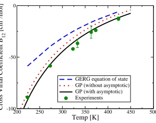
The CO2−CO PES is then used to compute the cross virial coefficient, taking the classical
contribution plus the (small) first-order quantum corrections; the calculation procedure has
been described previously28. A comparison with experimental data is shown in figure 5.
The PES produces accurate, first-principles, parameter-free prediction of this quantity, over
the range of temperatures studied experimentally. Also shown are the PES predictions with
200 250 300 350 400 450 500
Temp [K] -100
-50 0
Cross Virial Coefficient B
12
[cm
3 /mol]
[image:12.612.227.386.74.199.2]GERG equation of state GP (without asymptotic) GP (with asymptotic) Experiments
FIG. 5. The CO2−CO cross virial coefficient: comparison of the GP calculations with experimental
data24–26 and the GERG equation of state27.
mostly determined by the PES region controlled by the GP, with the long-range asymptotic
calculation making a small but significant further contribution. Also in figure 5 are the
results from the GERG model27, a widely used empirical equation of state. Despite the
extensive fitting involved in the development of the GERG equation of state, the predictions
of the present first-principles approach gives significantly better agreement with experiment.
V. FUTURE WORK
There are numerous extensions that follow from this approach. Application to many
other chemical systems is straightforward. Furthermore, the model’s performance for small
training set sizes could be optimised by sequentially adding training points through active
learning methods29. This could be achieved either with or without a priori knowledge of
the test data, depending on the potential energy data to be modelled. Another promising
application is the interpolation of non-additive potentials, which are known to be difficult
to fit30. Such data are usually high-dimensional, vary strongly and rather unpredictably
with geometry, and can have many symmetries. Finally, existing high-precision calculations
could be used as training and test data for interpolation by the algorithm. Here a sparse
GP31could select a subset of the preexisting data to train the model, leading to numerically
VI. CONCLUSIONS
The procedure described here produces intermolecular potential energy surfaces efficiently
from relatively few input data points. The algorithm is straightforward to generalise to
new molecular pairs. It uses a symmetric Gaussian process, with the inverse interatomic
distances as input variables. The GP is trained using data on a Latin hypercube design,
with a maximin criterion for the inverse internuclear distances.
The general utility and robustness of the approach have been demonstrated by testing
against three systems involving CO2, a system with a deep energy minimum (HF−HF) and
a system with 48 symmetries (CH4−N2). In all cases the approach accurately predicts an
extensive test data set, with no a priori knowledge, and gives RMSE values that are similar
to, or better than, the best fits in the literature, which were generally based on thousands of
training points. Furthermore, the interpolation method can be readily and directly applied
to any pairwise interaction, at least for simple molecules, with no bespoke work beyond
identifying the relevant symmetries. The approach contains two key features: the use of
in-verse interatomic distances as the GP input variables, and a strategy for positioning training
data on a Latin hypercube design with a maximin criterion on the inverse intermolecular
distances.
As the method requires only a relatively small number of training points it can be used
with more precise and computationally demanding potential energy calculations. An
exem-plar is CO2−CO, for which a four-dimensional PES was produced from 135 data points. This
CO2−CO PES was used to compute the cross virial coefficient, leading to parameter-free
predictions of this quantity that agree very well with experimental data.
SUPPLEMENTARY MATERIAL
See the supplementary material for fortran code for the CO2−CO PES used in section IV.
ACKNOWLEDGEMENTS
The authors are grateful to the EPSRC for the award of a studentship to EU, and to the
University of Nottingham for the use of the ‘Minerva’ high-performance computing facility.
compiled during the IMPACTS project.
Appendix A: Latin hypercube sampling
Latin hypercube (LHC) sampling is a method of choosing sampling points in a
multidi-mensional space. LHC sampling aims to spread the sample points more evenly across all
possible values than random sampling. In 2D a latin square is defined as a set of samples with
exactly one sample in each row and column. For a given number of rows and columns there
are many permutations that satisfy this. A LHC generalises this to an arbitrary number
of dimensions by requiring that each hyperplane normal to one of the co-ordinates contains
exactly one sample.
We generate an M dimensional unit LHC ofN sample points as follows.
• Place all N points on the diagonal of the hypercube to create an initial LHC. We
do this by placing the nth point so that each co-ordinate value lies in the range
(n−1)/N...n/N, with the value within the range being chosen randonly, uniformly
and independently for each co-ordinate.
• Choose two points at random and swap one of their co-ordinate values, chosen at
random. This permutes the sampling configuration, while ensuring we still have a
LHC, as defined above.
• Repeat the co-ordinate swaps until the desired number of swaps has been completed.
Appendix B: Latin hypercube generation
We wish to generate a dataset of model evaluations, {xi, f(xi)}Ni=1, that can be used to
train the Gaussian process, where the xi represent N distinct molecular geometries. Each
element ofxi is the inverse distance between two atoms, one from each of the molecules under
consideration. The design only needs to contain points in a symmetry-distinct subspace.
For example, in CO2-Ne the O nuclei are denoted O1 and O2, and the symmetry-distinct
subspace is defined such that Ne is always nearer to O1 than to O2. Space filling designs
are held to be good choices for Gaussian process models, and so we will use a maxi-min
the minimum distance between any two design points. Latin hypercube (LHC) designs are
used as candidate designs, as they naturally fill space to some extent, and we then choose a
preferred design from a large number of candidates. We define the effective distance between
points xi and xj in the design to be
|x|2ij = (xi−xj)>(xi−xj) (B1)
and we generate a training design using the following algorithm:
• Generate a LHC in 1/r and rigid-body rotation angles. (For non-rigid molecules,
intramolecular coordinates would also be used.)
• Convert the LHC data to atomic positions and compute all interatomic distances for
pairs of atoms on separate molecules.
• Reject the geometries that don’t obey the geometric constraint or lie outside the
symmetry-distinct region of coordinate space.
• Reject the entire LHC if it does not contain at least the target number of
geome-tries (usually the mean number of remaining points after the geometric constraint is
applied).
• Find the minimum|x|2
ij within the current LHC.
• Repeat for as many new LHCs as desired and return the LHC with the largest minimum
|x|2
ij.
Appendix C: Symmetric covariance function
The motivating problem is modelling the H2 - CO2 system, which we parameterise by 6
distances:
• r1 = H1 → C
• r2 = H2 → C
• r3 = H1 → O1
• r5 = H1 → O2
• r6 = H2 → O2
The potential function f between the two molecules obeys the following symmetry
rela-tions
f(123456) =f(214365) =f(125634) =f(216543)
where f(123456) denotes f(r1, r2, r3, r4, r5, r6).
In other words, the function
f(x) = f(σx)∀σ∈K4
where K4 is the permutation group consisting of the permutations
σ1 = (12)(34)(56), σ2 = (35)(46) σ3 = (12)(36)(45)
where we are using cyclic notation for the permutations. Note that along with the identity
e, these four permutations form an abelian group that is isomorphic to the Klein-4 group
K4 (≡Z2×Z2), i.e., σi2 =e and σ1σ2 =σ3 etc.
1. A single symmetry
To illustrate the procedure, suppose we want to model f where f is invariant under the
single permutation σ, whereσ2 =e. If we assume
f(x) = g(x) +g(σx)
for some arbitrary function g, then f has the required symmetry. If we model g(·) ∼
GP(0, k(·,·)), then the covariance function for f is
kf =Cov(f(x), f(x0))
=k(x, x0) +k(σx, x0) +k(x, σx0) +k(σx, σx0)
If k is an isotropic kernel (we only actually require isotropy for each pair of vertices that
swap inσ), thenk(x, x0) =k(σx, σx0) and k(x, σx0) = k(σx, x0) as swaps only occur in pairs
kf(x, x0) =k(x, x0) +k(σx, x0)
saving half the computation.
2. Invariance under permutations in K4
Now consider functions that are invariant to permutations in K4. If we write
f(x) =g(x) +g(σ1x) +g(σ2x) +g(σ3x)
then if g(·)∼GP(0, k(·,·))
kf(x, x0) =k(x, x0) +k(σ1x, x0) +k(σ2x, x0) +k(σ3x, x0)
+k(x, σ1x0) +k(σ1x, σ1x0) +. . . k(σ3x, σ3x0)
(C1)
If k is isotropic, then k(x, σix0) = k(σi−1x, x0). Thus k(x, x0) = k(σix, σix0), k(x, σix0) =
k(σix, x0) andk(σix, σjx0) =k(σkx, x0) for i6=j 6=k. Thus we can use
kf(x, x0) =k(x, x0) +k(σ1x, x0) +k(σ2x, x0) +k(σ3x, x0)
as a covariance function for f instead of Equation (C1). This reduces the amount of
com-putation needed to calculate the covariance functions by 75%.
Note that we don’t need k to be completely isotropic for this simplification to hold, only
that the covariance function is isotropic for any pair of inputs that swap in any of the
permutations. So in the H2−CO2 system, we require the length-scales to be the same for
inputs 1 and 2, and the same for inputs 3, 4, 5 and 6.
REFERENCES
1D. Silver, A. Huang, C. J. Maddison, A. Guez, L. Sifre, G. V. D. Driessche, J.
Schrit-twieser, I. Antonoglou, V. Panneershelvam, M. Lanctot, S. Dieleman, D. Grewe, J. Nham,
N. Kalchbrenner, I. Sutskever, T. Lillicrap, M. Leach, K. Kavukcuoglu, T. Graepel, and
D. Hassabis, Nature 529, 484 (2016).
2R. Chen, E. Jiao, H. Zhu, and D. Xie, Journal of Chemical Physics 133, 104302 (2010).
4R. Hellmann, E. Bich, E. Vogel, and V. Vesovic, Journal of Chemical Physics 141, 224301
(2014).
5Y. Cui, H. Ran, and D. Xie, Journal of Chemical Physics 130, 224311 (2009).
6G. S. Kimeldorf and G. Wahba, Ann. Math. Statist. 41, 495 (1970).
7C. Rasmussen and C. K. I. Williams, Gaussian Processes for Machine Learning (MIT
Press, 2006).
8T.-S. Ho and H. Rabitz, Journal of Chemical Physics 113, 3960 (2000).
9A. P. Bartok and G. Csanyi, Int. J. Quant. Chem. 115, 1051 (2015).
10A. P. Bartok, M. C. Payne, R. Kondor, and G. Csanyi, Phys. Rev. Letts. 104, 136403
(2010).
11W. J. Szlachta, A. P. Bartok, and G. Csanyi, Phys. Rev. B 90, 104108 (2014).
12M. Rupp, M. R. Bauer, R. Wilcken, A. Lange, M. Reutlinger, F. M. Boeckler, and
G. Schneider, J. Chem. Phys. 136, 074102 (2012).
13A. P. Bartok, M. J. Gillan, F. R. Manby, and G. Csanyi, Phys. Rev. B 88, 054104 (2013).
14C. M. Handley, G. I. Hawe, D. B. Kell, and P. L. A. Popelier, Phys. Chem. Chem. Phys.
11, 6365 (2009).
15M. J. Mills and P. L. Popelier, Computational and Theoretical Chemistry 975, 42 (2011).
16M. J. L. Mills, G. I. Hawe, C. M. Handley, and P. L. A. Popelier, Phys. Chem. Chem.
Phys. 15, 18249 (2013).
17T. L. Fletcher and P. L. Popelier, Chemical Physics Letters 659, 10 (2016).
18H. J. Werner et al., “MOLPRO version 2012.1: A package of ab initio programs,”
http://www.molpro.net (2012).
19“GPy: A Gaussian Process framework in python,” http://github.com/SheffieldML/GPy
(2012–2015).
20This can be obtained from the maximum energy, before applying the energy cut-off, over
the test data (if available) or training data.
21A. C. Legon and A. P. Suckley, J. Chem. Phys. 91, 4440 (1989).
22K. deLange and J. R. Lane, J. Chem. Phys. 134, 034301 (2011).
23S. Sheybani-Deloui, A. J. Barclay, K. H. Michaelian, A. R. W. McKellar, and N.
Moazzen-Ahmadi, J. Chem. Phys. 143, 121101 (2015).
24T. L. Cottrell, R. A. Hamilton, and R. P. Taubinger, Trans. Faraday Soc.52, 1310 (1956).
26B. Mallu, G. Natarajan, and D. Viswanath, The Journal of Chemical Thermodynamics
21, 989 (1989).
27O. Kunz, R. Klimeck, W. Wagner, and M. Jaeschke,The GERG-2004 wide-range reference
equation of state for natural gases (Fortschr.-Ber. VDI, VDI-Verlag, D¨usseldorf, 2007).
28M. P. Hodges, R. J. Wheatley, G. K. Schenter, and A. H. Harvey, J. Chem. Phys. 120,
710 (2004).
29J. Beck and S. Guillas, arXiv (2014), 1410.0215v2.
30M. T. Oakley and R. J. Wheatley, J Chem Phys 130, 034110 (2009).
31E. Snelson and Z. Ghahramani, in Advances in Neural Information Processing Systems 18