Fluid structure behaviour in gas oil two phase flow in a moderately large diameter vertical pipe

* _{Corresponding author. Tel.: +44 (0)115 9514178}

E-mail address: [email protected] (Buddhi Hewakandamby).

Fluid structure behaviour in gas-oil two-phase flow in a moderately large

diameter vertical pipe

Rajab Omar 1_{, Buddhika Hewakandamby} 1,*_{, Abdelwahid Azzi} 2 _{and Barry Azzopardi} 1

1 _{Faculty of Engineering, University of Nottingham, University Park, Nottingham NG7 2RD, United Kingdom}

2 _{Université des Sciences et de la Technologie Houari Boumedien, LTPMP/FGMGP, BP 32 El Alia, Algiers}

16111, Algeria

Abstract

Intermittent flows in vertical pipes occur in many industrial settings including power

generation and downstream oil-and gas production. This type of flows include cap bubble, slug

and churn flow regimes. These regimes are of interest as downstream processes and control

may heavily depend on the intermittency of the inflow. There are a number of correlations that

predicts the features in such flows in vertical pipes. Most of the correlations were developed

for air and water fluid pair for slug flow regime in vertical pipes with 25 to 50 mm inner

diameter. In this paper, an attempt has been made to assess the suitability of several of these

correlations specific to slug flow regime for a fluid pair that is different to air-water system. In

this work, air-silicone oil flow development was experimentally investigated in a vertical pipe

with an inner diameter of 68mm. A Wire Mesh Sensor (WMS) and an Electrical Capacitance

Tomography (ECT) sensor were installed in series at four locations (15D, 30D, 45D and 65D)

downstream of the mixing section. The flow was visually observed using a high speed camera.

The void fraction time series obtained from the WMS and the ECT were used to establish the

flow characteristics such as slug length, slug frequency, void fraction in liquid slugs and Taylor

bubble velocity. A comparison showed that the void fraction measurements using ECT and

WMS are in good agreement. Axial measurements shows that the flow development beyond

2

deviation associated with the existing slug flow models, particularly those developed to predict

the gas holdup in liquid slugs.

3 1 Introduction

Situations where gas and liquid flowing simultaneously in vertical pipes are of importance to

many process industries due to the flow patterns they produce depending on pipe diameters,

flow rates and fluid properties. This poses a considerable challenge not only in designing such

plants but also in controlling the processes. The intermittency in phases at the receiving end

influences the choice of equipment as well as downstream process conditions. Over the time

there have been many investigations focussed on developing robust models to predict the

intermittent nature of gas liquid two phase flows (Khatib and Richardson, 1984; Barnea and

Brauner, 1985; and Brauner and Ullmann, 2004). Most of the correlations were developed from

data gathered using air and water as the fluids and pipe diameters around 25 or 38 mm pipes.

This paper presents an attempt to assess the applicability of several of these correlations on

larger pipe diameter with a liquid phase different to water.

Co-flowing gas and liquid in a pipe would arrange themselves depending on the flow rates,

fluid properties and pipe geometries such as diameter and the inclination angle of the pipe. For

the vertically upward flow, these configurations are mainly, bubbly, slug, churn and annular

flows. Transition from one flow regime to another, which is due to the variation of the flow

parameters and pipe layout geometry and the forces acting on the phases are of primary interest.

Local measurements of flow parameter at different locations in co-current gas-liquid flow are

desirable for development and validation of computational fluid dynamics (CFD) codes.

Reliable two-phase flow data is required for developing flow models and confirming the

existing models. The characterisation of axial flow evolution has a crucial industrial

application, especially in gas and oil industry where the transition between flow patterns has a

4

Among the flow regimes, it is important to investigate the intermittent slug flow as it can cause

severe damage to the installation. This is due the cyclic forces it could exert on the pipe and

the structural supports that hold the pipes. In vertical upward flow, the intermittency appears

as periodic units. Each unit is formed by a bullet gas bubble with a diameter almost equal to

that of the pipe; the remaining space is filled with liquid. This bubble called Taylor bubble is

followed by a small gas bubbles lying in the continuous liquid phase.

Since the early studies of Dumitrescu (1943) and Davies and Taylor (1950), a large volume of

work, both experimental and numerical, has been carried out to analyse and characterize the

slug flow regime (Taitel and Barnea, 1990; and Fabre, 2003). An analysis of the available

literature shows that, with very few exceptions, all the investigations were achieved using

air-water mixture and on laboratory size scale.

The models developed based on such data are devoid of the dependency on the physical

properties of the process fluids used in many industrial settings. This has raised the demand of

experiments that employ fluids with viscosity, density and surface tension different to that of

water. Thereby the experiments presented in this work were designed to provide a more

accurate and high-resolution database of measurements made utilising advanced

instrumentations on an oil with physical properties close to that of industrial fluids. This data

will expand the range of published results and could be used to evaluate the available flow

transition models.

In this work, the axial flow development in 4.5 m long riser with 68 mm internal diameter (ID)

is examined along with the characterisation of slug flow regime. The results describe how the

flow structures in the vertical section develop as it moves downstream of the mixer. It also

5

silicone oil experiments were conducted at ambient pressure and temperature for 60 different

flow combinations.

2 Experimental arrangement and procedure

2.1 Flow facility description

The two-phase air-silicone oil flow experiments were conducted in the flow rig illustrated in

Figure 1. The flow facility consists mainly of a liquid tank, a centrifugal pump, a mixing

section, a vertical riser, a cyclone separator. Furthermore, air and liquid flow meters, electronic

temperature sensors and pressure transmitters were implemented on the rig for measurements.

The main Perspex pipe section has an average internal diameter of 68mm, while the air and the

liquid inlets to the mixing section are 28 mm and 42 mm diameter respectively.

During the experiments, the silicone oil is pumped from the storage tank using the centrifugal

pump into the mixing section. A bypass line is installed for a better liquid flow control and also

to boost the flow stability. The air is supplied from a central compressed air line. Temperature

and pressure of both the liquid and the gas streams are measured prior to the mixing section by

electronic temperature sensors and pressure transmitters respectively. The silicone oil and air

are well mixed within the mixing section and then the mixture flows along a vertical riser of

4.5 m length before it reaches the horizontal section. This offers 66 pipe diameter length which

can be enough for the flow development (Azzi and Friedel, 2005; Benbella et al., 2009; and

Abdulkadir et al., 2012). The two-phase flow in the vertical section is passed into the horizontal

test section before it is returned to the holding tank where the phases are separated. The air is

vented into the atmosphere while the silicone oil is returned to the bottom of the storage tank

prior to its reuse.

The time series of the averaged void fraction was obtained at four different locations (15, 30,

6

mainly presented in this paper, since there was intangible change in the void fraction signal at

45 and 65 pipe diameter. For all experiments, the Wire Mesh Sensor (WMS) was placed

immediately after the Electrical Capacitance Tomography (ECT) sensor to eliminate the impact

of the intrusive nature of the former. It should be noted that the WMS is an intrusive technique

that might cause distortion of the flow structures and bubble fragmentation, thus it is usually

installed downstream of the non-intrusive ECT system.

Figure 1: The schematic diagram of the flow facility.

2.2 Measurement techniques

Electrical Capacitance Tomography (ECT) which is described in detail by Hammer (1983)

and Huang (1986) and the Wire Mesh Sensor tomography (WMS), that introduced by Prasser

et al. (1998) and developed for capacitance measurement by Da Silva et al. (2007), were used

to obtain real-time void fraction measurements in these experiments. These measurements 15D

7

techniques have been extensively tested over the last decade and proved to be accurate within

acceptable margins (Azzopardi et al., 2010; Sharaf et al., 2011; and Banowski et al., 2016).

To investigate the two-phase flow evolution, experiments are designed using ten gas superficial

velocities in conjunction with six liquid phase superficial velocities giving a total of 60

conditions. The gas and liquid superficial velocities were varied from 0.045 to 3.2 m s-1 _and from 0.15 to 0.53 m s-1 respectively. A data acquisition system using LabVIEW software was developed for simultaneous acquisition of data from all devices. A trigger signal from the WMS

is used to initialise the ECT and the other measuring devices including flowmeters.

During each experiment, the flow rate, pressure, temperature and void fraction were measured

after allowing the flow to stabilise. The process was repeated for each run until the full set of

experiments was completed.

The consistency of the results was checked through data analysis process which included

computing the probability density functions (PDF), frequency and structure velocities.

Detailed analysis of the void fraction time series signal (as described in section 3) was

performed. The characteristic parameters are reported including, cross-sectional averaged void

fraction, probability density functions, structure frequency and velocity, slug length, Taylor

bubble velocity, and the void fraction in the body of slugs. The available flow models and

existing empirical correlations were tested using the experimental data at 45D downstream of

the mixer, where the flow is considered developed.

3 Data processing

The instrumentations that were used in this work such as capacitance WMS and ECT system

8

along the vertical pipe. Real-time measurements in the form of void fraction time series were

obtained from both sensors.

The obtained voltage signals from WMS and ECT system were converted to void fraction data

utilising a calibration routine. The time series of the void fraction distribution was used to

estimate several flow parameters including the probability density functions (PDFs), radial

void fraction, bubble size distribution, structure frequency and structure velocity.

3.1 Probability density function

Probability density functions (PDF) shows how often each value of void fraction occurs within

a particular range. PDFs plots show the rate of change of probability with void fraction values,

where the total area under PDFs plot should be equal to one. The PDFs has been widely used

to identify the relevance flow patterns. The work of Jones and Zuber (1975) demonstrates the

ability of this statistical property to discriminate between the main flow patterns. In addition,

PDFs can also be used to estimate different flow parameters such as film thickness, slug length

and bubble length in slug flow (Costigan and Whalley, 1997).

The PDFs plots of the cross-sectional averaged void fraction are used to categorise the

corresponding flow patterns based on the work of Jones and Zuber (1975) and Costigan and

Whalley (1997) in which they pointed out that the PDFs of the void fraction data can be used

to quantitatively discriminate the main flow patterns. Bubbly flow is associated with a single

peak at low void fraction, while a broad single peak at high void fraction and a tail stretched to

low void fraction represents churn flow. Slug flow, the intermittent flow pattern between

bubbly and churn flow, is identified by a twin peak PDF, one at low void fraction corresponding

to the void fraction in liquid slug and the other at high void fraction representing Taylor bubble.

The PDF of the cross-sectional averaged void fraction was computed by taking into account

9

measurement period. For this paper, we have considered 100 bins between 0 and 1 for the void

fraction data.

3.2 Structure Frequency

The power spectral density (PSD) method was applied to obtain the frequency of the time series

data that describe the periodicity of the flow structures such as slugs. The PSD was estimated

through discrete Fourier transform of the autocorrelation of the time series. Fourier analysis

transforms the void fraction data form its time domain to the frequency domain as shown in

equation Error! Reference source not found..

𝑆_𝑥𝑥(𝑓) = ∫_−∞+∞𝑅_𝑥𝑥(𝜏)𝑒−𝑗2𝜋𝑓𝜏_{𝑑𝜏 (1)}

where; 𝑅𝑥𝑥 is the autocorrelation function of the void fraction time series while 𝑆𝑥𝑥(𝑓) is the

power spectral density as reported by Bendat and Piersol (1980).

The frequency of the structures was also estimated using the method proposed by Hazuku et

al. (2008) for large disturbance waves. The void fraction signal from the WMS and ECT was

used to estimate the front and the tail of Taylor bubble. A Taylor bubble is defined as a part of

the void fraction signal whose peak is higher than the upper average of the void fraction and

both ends are lower than the average of the void fraction as described by Hazuku et al. (2008).

The part of the signal between two trailing Taylor bubbles represents liquid slug. The results

were in a good agreement with the manual counting and the PSD method.

3.3 Structure velocity

The structure velocity was determined by cross correlating the void fraction time series

obtained from the twin-plane ECT sensor. Cross correlation function is simply the sliding dot

product of the two time series from the two ECT planes to estimate the time delay 𝜏 between

10

represent the signal at the first and second plane of the ECT system respectively. Thus the

cross-correlation is given by

𝑅𝑥𝑦(𝑡, 𝑡 + 𝜏) =_𝑁1 ∑𝑁𝑖=1𝑥(𝑡𝑖)𝑦(𝑡𝑖+ 𝜏) (2)

where N is the number of samples in each time series. It produces the time delay of a signal

which is equal to the distance divided by the propagation velocity. Since the distance between

the planes of the sensors is known, the structure velocity is merely equal to the distance between

the two sensors divided by the time delay estimated from the cross-correlation.

3.4 Slug length

The length of slugs was estimated using the averaged transitional velocity of slugs and the

resident time of slugs at the measuring plane. The velocity was assumed to be constant

throughout the test section and the following equation was used to determine the slug length.

𝐿_𝑠 = 𝛥_𝑡 . 𝑈_𝑠 (3)

Where; 𝐿𝑠 is the slug length, 𝛥𝑡 is the resident time of slugs at the sensor and 𝑈𝑠 is the velocity

of slugs.

All mathematical operations are implemented in MATLAB, is some cases, using embedded

routines within the software.

4 Results and discussion

4.1 Comparison between WMS and ECT performance

Electrical Capacitance Tomography (ECT) and Wire Mesh Sensor (WMS) tomography have

been widely tested for multiphase flow applications over the last decade. For instance WMS

measurements showed good agreement with X-ray tomography and Gamma radiography for

void fraction measurements as reported by Prasser et al. (2005) and Prasser (2000). Whereas

11

they also highlighted the advantage of each technique. For all experiments reported in this

work, the WMS was placed downstream of the ECT sensor in order to minimise the intrusive

nature of the WMS and also to limit the change in the vertical distribution of the void fraction

between the two measuring planes.

The void fraction data gathered from both sensors showed a reasonable agreement for all

experiments. Figure 2shows PDFs of the cross section averaged void fraction time series data

simultaneously collected using WMS and ECT at the given flow conditions. The comparison

illustrates that at liquid superficial velocity, Uls, 0.22 m s-1 and gas superficial velocities, Ugs, 0.045 m s-1 and 0.18 m s-1, the PDF corresponds to bubbly flow (Figure 2-a) and cap bubble (Figure 2-b) respectively. For these flow patterns, the WMS seems to give higher void fraction

which might be due to the drag effects triggered by the intrusive nature of the sensor, where at

low flow rates the bubbles decelerate at the measuring plane causing an increase in average

void fraction.

Figure 2: PDF plots of the cross-sectional averaged void fraction for ECT and WMS at 45 ID downstream the mixer. The liquid superficial velocity = 0.22 m s-1_.

(a) U_gs=0.045 m/s (b) U_gs=0.18 m/s

(c) U_gs=0.55 m/s _{(d) U}

gs=3.21 m/s Bubbly

Cap bubble

12

At gas superficial velocity, Ugs 0.55m s-1 (Figure 2-c), both sensors show almost similar PDF plots which indicate slug flow. For the maximum flow condition achievable in these

experiments (Uls=0. 22m s-1, Ugs=3.21m s-1) (Figure 2-d), the PDF signatures for ECT and WMS characterise churn flow, where ECT provides a higher peak at slightly higher void

fraction than the WMS. It is obvious that the difference between the PDF plots created using

the two sensors reduces as the gas superficial velocity increases. Generally, the PDF signature

for both devices indicates similar flow patterns. The results showed a good agreement between

both sensors, for the full range of flow conditions, with an average percentage error of 5% and

standard deviation of 1.02, while the averaged absolute percentage error is 6.7% in void

fraction measurements.

Figure 3: Radial void fraction profile and bubble size distribution obtained from WMS at 45D downstream of the mixer. Liquid superficial velocity = 0.22 m.s-1_.

The radial void fraction profiles and bubble size distributions at different gas superficial

velocities are illustrated inFigure 3. The radial distribution of gas fraction shows a flat profile

0 0.5 1

0 0.01 0.02 0.03 0.04 0.05 [r/R] V o id f ra c ti o n 0 5 10 15 20 25

0 20 40 60

0 0.5 1 1.5 2 2.5 3 3.5 4 4.5 D

b (mm)

  /  D b ( % /m m ) 0.045 0.18 0.55 3.21

Gas superficial velocity,m/s

13

at low gas superficial velocity (Ugs=0.045 m s-1). This corresponds to a dispersed bubbly flow, in which small gas bubbles are uniformly distributed throughout the cross section of the pipe.

As the gas superficial velocity increases, the uniform distribution disappear and the radial void

profile tends to indicate a local maxima at the core of the pipe. At these conditions large bubbles

are formed and rapidly shifted to the centre of the pipe. At Ugs = 0.18 m s-1 and 0.55 m s-1 the bubble size distribution switched from single to bimodal, indicating the transition to cap bubble

and slug flow regime respectively. The most significant observation from these results is that

the bubble sizes at the measuring plane are greater than the wire spacing of the WMS and hence

the error due to the sub-resolution bubble sizes is considered to be minimum. This is expected

since the initial bubble size is 3mm while the spatial resolution of the sensor is 2.8 mm. It

seems that small bubbles are deaccelerated at the sensor wires while the large bubbles are

accelerated as reported by Ito et al. (2011). This hypothesis explains the reduction in the

difference between the two sensors as the gas superficial velocity increases.

Banowski et al. (2016) suggested the best working range for the WMS. They also reported that

the sensor insensitiveness of small bubbles could be overcompensated by the deceleration of

bubbles at the crossing point. Therefore, in this case, the WMS is expected to overestimate the

averaged void fraction at a low gas flow rate. On the other hand, the limited spatial resolution

of the ECT sensor should not be ignored. It is a non-invasive sensor and hence the void fraction

at the core of the pipe may not be accurately represented, especially when the gas phase is not

uniformly distributed. On the other hand, a twin plane ECT system can provide velocity

information without altering the flow structure.

In conclusion, it can be said that both sensors can give an acceptable and comparable estimation

of the cross-sectional average void fraction. The high temporal and spatial resolution of the

WMS in comparison to ECT sensor can provide detailed information of the flow and can detect

14

structure velocity without disturbance of the flow. Both sensors have strengths and weaknesses

due to the limitations in their respective designs and it is difficult to select one over the other.

It is obvious that if both sensors are integrated, a considerable amount of flow information can

be obtained.

4.2 Cross-sectional averaged void fraction

Figure 4 illustrates the cross-sectional averaged void fraction at Uls = 0.3 m s-1 at four axial locations along the test section. It should be noted that the difference in averaged void fraction

at 45D and 65D is small and within the uncertainty margin for the measurements. The PDF

plots at 45D and 65D are identical in shape and no change in the flow structures was observed.

Therefore, the changes due to flow development are considered to be insignificant at those

locations.

Figure 4: Mean void fraction at four axial locations at liquid superficial velocity, Uls = 0.3 m s-1.

The superficial gas velocity has a significant influence on the subsequent flow development in

the riser. Figure 5 shows the mean void fraction for the range of gas and liquid flow rates 45D

downstream of the gas injection point. The curves indicate a continuous increase in the void

0 0.5 1 1.5 2 2.5 3 3.5

0 0.2 0.4 0.6 0.8 1

Gas superficial velocity(m/s)

V

o

id

f

ra

c

ti

o

n

15

fraction with increasing superficial gas velocity. It can be seen that the void fraction is sensitive

to the change of superficial gas velocity at low values. Figure 5 clearly indicates that the curves

tend to level off beyond the superficial gas velocity 1.5 m s-1. This trend can be interpreted as the change in flow patterns with the increase of superficial gas velocity. The transition from

bubbly to slug flow is associated with a considerable shift in the rate of change of the void

fraction, w.r.t. the superficial gas velocity. The higher gradient up to Ugs = 0.55 m s-1 explains bubbly flow, whereas the transition from slug to churn incorporates a slight change in the rate

of change of void fraction beyond Ugs > 0.91 m s-1.

Figure 5: Variation of the averaged void fraction with superficial gas velocity for several liquid superficial velocities at 45D.

The influence of superficial liquid velocity on the mean void fraction shows a decrease in the

void fraction as the liquid superficial velocity increases. However, it can be mentioned that the

superficial liquid velocity has a weak influence on the void fraction comparing to that of

superficial gas velocity.

0 0.5 1 1.5 2 2.5 3 3.5

0 0.2 0.4 0.6 0.8

Gas superficial velocity(m/s)

V

o

id

f

ra

c

ti

o

n

0.15 0.22 0.30 0.38 0.45 0.53

16 4.2.1 Void fraction estimation

Void fraction is a crucial parameter in characterising two-phase flow. Therefore an accurate

prediction of void fraction is of great interest in industrial applications. In this work, Drift-flux

model was used to estimate the void fraction in the region of slug flow. Drift-flux model

considers the mixture as whole, instead the two-phase separately. The one-dimensional

drift-flux model, that was introduced by Zuber and Findlay (1965) and developed by Wallis (1969)

and Ishii (1977), is widely used to estimate the averaged void fraction. It is usually preferred

over the two-fluid models for its simplicity and applicability in a wide range of flow conditions.

The general form of the one-dimensional drift-flux model is represented by equation Error! Reference source not found..

𝜀𝑑 = _𝐶 𝑈𝑔𝑠

0𝑈𝑚+𝑈𝑑 (4)

Average void fraction is given by 𝜀_𝑑while 𝑈_𝑑 and 𝐶₀ are the drift velocity and distribution

parameter respectively. The drift velocity is the relative velocity between the gas phase and

mixture velocity at the centreline. The distribution parameter represents the relative velocity of

the gas phase in Taylor bubble to the mixture velocity of slug unit. The drift velocity is

estimated by the equation proposed experimentally by Nicklin et al. (1962) which is given by

the equation Error! Reference source not found. which is in agreement with the theoretical work of Dumitrescu (1943) and Davies and Taylor (1950).

𝑈_𝑑 = 0.35√𝑔𝐷 (5)

where g is the gravitational constant and D is the internal diameter of the pipe. The distribution

parameter 𝐶0 was found to have different values with respect to the corresponding flow

patterns. For slug flow it is widely acceptable that 𝐶0 is equal to 1.2, however in this work the

17

𝐶₀ = (1.2 − 0.2√𝜌𝑔

𝜌𝑙) (6)

The symbols 𝜌_𝑔 and 𝜌_𝑔 represent the density of gas and liquid respectively. The Drift-flux

model results were compared to the experimentally measured averaged void fractions at 15D,

45D, and 65D downstream of the mixing section as presented in Figure 6. The predicted void

fraction at 45D and 65D is almost identical. The figure shows a reasonable agreement between

the predicted and experimental data with an average percentage error of -2.38 and standard

deviation of 0.6. The accuracy of the model decreases for data obtain closer to the mixing

section. For instance, at 15D, the cross-sectional void fraction data was visibly under predicted

with an average percentage error of -8.5 and standard deviation of 0.6. It is evident that highly

aerated underdeveloped slugs were more dominant at 15D from the mixing section leading to

underestimation of the void fraction. As the slugs move upward towards 45D and 65D

downstream of the mixer, developed slugs become more frequent leading to improved accuracy

of the predicted data. Since the change in the averaged void fraction and the flow structure at

45D and 65 D was insignificant, and also there is no recognisable difference in the flow

structures at 45D and 65 D, The flow is considered as developed at 45D and beyond. Therefore,

to minimise the number of experiments and to minimize the experimental costs, measurements

18

Figure 6: Comparison of experimentally measured void fraction and predicted void fraction using drift flux model at 15D and 45D downstream of the mixer.

4.3 Flow patterns identification

The PDF signatures of the cross-sectional averaged void fraction, obtained from the WMS and

ECT, are used to identify the corresponding flow patterns. Visual observations corroborated

the statistical analysis and have been widely used to discriminate the main flow patterns

qualitatively. The main flow patterns observed in the riser are bubbly, cap bubbles, slug and

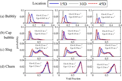
churn. Figure 7 shows the time series of the main flow pattern and their PDFs for gas superficial

velocity ranges from 0.45 to 3.21 m.s-1 _{and liquid superficial velocities from 0.15 to 0.53 m.s} -1_{. The results show that each flow regime has a unique probability density function distribution} comparable to those reported in the literature.

0 0.2 0.4 0.6 0.8 1

0 0.2 0.4 0.6 0.8 1

P

re

d

ic

te

d

v

o

id

f

ra

c

ti

o

n

Measured void fraction 15D

19

Figure 7: Cross-sectional averaged time series of void fraction and the corresponding PDFs for each flow pattern.

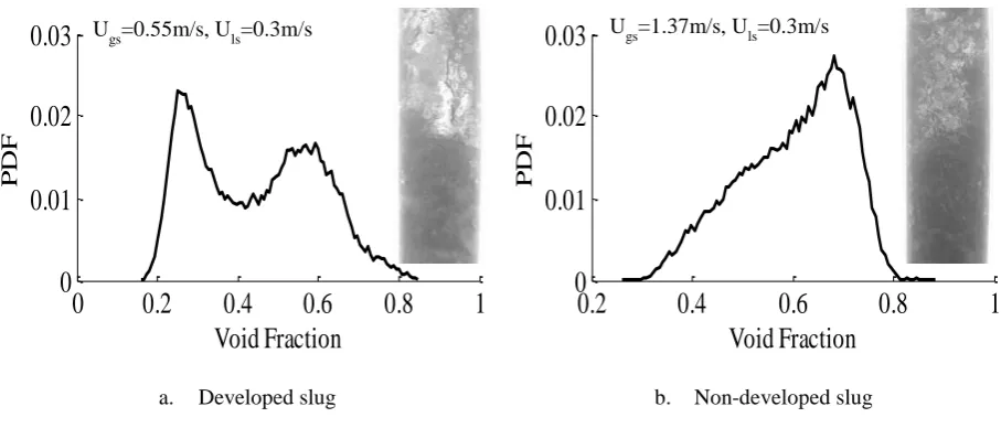
According to Costigan and Whalley (1997), slug flow is identified by twin peak PDF, one at

low void fraction corresponding to the smaller bubbles in the liquid slug, while the other at

high void fraction corresponding to the Taylor bubble. The most remarkable observation in

the riser was the non-developed slugs; they are short and highly aerated slugs, similar to those

reported by Nydal et al. (1992) in horizontal pipes. Non-developed slugs in the riser are more

likely to occur near the transition to churn flow at high gas flow rates. This type of slug is

characterised by a single wide peaked PDF. Therefore it can be inaccurately identified as churn

flow. Figure 8 illustrates the difference between developed slugs and non-developed slugs.

0 0.2 0.4 0 0.4 0.8 0 0.5 1

0 2 4 6 8 10

0 0.5 1 Time (sec) V o id f ra c ti o n

0 0.2 0.4 0.6

0 0.05 0.1

Bubbly

0 0.2 0.4 0.6 0.8

0 0.05 0.1

Cap bubble

0 0.5 1

0 0.01 0.02

Slug

0 0.5 1

20

Figure 8: Probability density function of a developed slug and a non-developed slug.

4.4 Flow transition along the axial direction

Void fraction measurements at three different locations downstream of the mixing section were

conducted. Void fraction information at each location is obtained using the ECT and the WMS

measurement probes.

It can be seen from Figure 9 that at lowest gas superficial velocity (case (a)), the averaged void

fraction near the mixer (at 15D) is the highest, while at the second location, 30D, it records the

lowest void fraction before increasing again at 45D downstream the mixer. Since the PDF plots,

as well as the visual observation, indicate bubbly and cap bubble flow, it can be reasoned that

at low gas superficial velocity, finer bubbles form near the mixer resulting dispersed bubbly

flow. Furthermore, the bubble density is high making the mixture to appear like a foam. As

the bubbles move up to the second position, 30D, larger ellipsoidal bubbles formed due to

coalescence and these bubbles moves to the centre of the pipe occupying a smaller area of the

cross section of the pipe. The observation is in agreement with Prasser et al. (2002) and Lucas

et al. (2005) for multi-disperse bubbles and Tomiyama (1998) for a single bubble. As the large

bubbles move upward at relatively higher velocity, more coalescence occurs forming larger

cap bubbles and hence the void fraction increases again.

0

0.2

0.4

0.6

0.8

1

0

0.01

0.02

0.03

Void Fraction

P

D

F

0.2

0.4

0.6

0.8

1

0

0.01

0.02

0.03

Void Fraction

P

D

F

U_gs=0.55m/s, U_ls=0.3m/s U_gs=1.37m/s, U_ls=0.3m/s

21

Figure 9: PDF plots for different flow condition at 15D, 30D and 45D downstream the mixer.

PDF plots were generated for superficial gas velocities 0.045 m s-1, 0.18 m s-1, 0.55 m s-1, and 3.21 m s-1 and superficial liquid velocities 0.22 m s-1, 0.38 m s-1, 0.53 m s-1 at selected axial positions. The flow pattern changes with different combinations of the liquid and gas

superficial velocities as shown in Figure 9 (a-d). Several flow patterns such as bubbly (Figure

6-a), cap bubbles (Figure 6-b), slug (Figure6-c) and churn (Figure 6-d) could be attained in the

riser. As the gas superficial velocity increases, the PDFs produced for the three measurement

locations are almost similar. It seems that at high gas flow rates, the change in the averaged

void fraction along the axial length is insignificant thus the required length for flow

development is expected to be shorter under these conditions. However, the interaction

between phases is considered to continue in risers, regardless their length, due to the change in

pressure and forces acting on bubbles.

0 0.2 0.4 0.6

0 0.05 0.1

Uls=0.22 m s-1

Ugs=0.045 m s-1

0 0.2 0.4 0.6

0 0.05 0.1

Uls=0.38 m s-1 Ugs=0.045 m s-1

0 0.2 0.4 0.6

0 0.05 0.1

Uls=0.53 m s-1 Ugs=0.045 m s-1

0 0.5 1

0 0.05 0.1

Uls=0.22 m s-1 Ugs=0.18 m s-1

0 0.5 1

0 0.05 0.1

Uls=0.38 m s-1 Ugs=0.18 m s-1

0 0.5 1

0 0.05 0.1

Uls=0.53 m s-1 Ugs=0.18 m s-1

0 0.5 1

0 0.02 0.04

Uls=0.22 m s-1 Ugs=0.55 m s-1

0 0.5 1

0 0.02 0.04

Uls=0.38 m s-1 Ugs=0.55m s-1

0 0.5 1

0 0.02 0.04

Uls=0.53 m s-1 Ugs=0.55 m s-1

0 0.5 1

0 0.02 0.04 Void Fraction p ro b a b il it y

Uls=0.22 m s-1

Ugs=3.21m s-1

0 0.5 1

0 0.02 0.04

Uls=0.38 m s-1

Ugs=3.21 m s-1

0 0.5 1

0 0.02 0.04

22

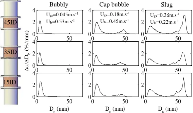
4.4.1 Bubble size distribution and radial void fraction

Bubble size distribution is obtained from WMS data using the algorithm developed by Prasser

et al. (2001). It is based on the gas volume fraction contained in each class of bubbles instead

of the number of bubbles. Figure 10 illustrates the bubble size distribution at three different

flow conditions. The x-axis denotes the volume equivalent bubble diameter (Db) and the y-axis denotes the ratio of the gas fraction per bubble class (Δ) to the equivalent diameter of the

bubble class (ΔDb).

Figure 10: Bubble size distribution for different flow patterns at three axial locations along the test section.

It is obvious that in the bubbly flow region the distribution displays a single peak at small

bubble size, this peak is shifted to the right as the bubbles move upwards in the column

indicating the bubble coalescence. At bubble/cap bubble transition, the distribution for the first

location shows a single peak indicating small bubble sizes and a long tail extended to relatively

large bubble sizes. This represents a nonhomogeneous bubbly flow. As the flow develops in

the axial direction, a second peak becomes apparent. This peak shows that large cap bubbles

become more frequent. It is clear that the estimated diameter of these bubbles is around 50 mm,

slightly below the pipe diameter. In slug flow region, the bubble size distribution is

45ID 35ID 15ID 0 50 0 2 4 D

b (mm)

  /  Db ( % /m m ) 0 50 0 2

40 50

0 2 4 0 50 0 2 4 D

b (mm)

0 50

0 2

40 50

0 2 4 0 50 0 2 4 D

b (mm)

0 50

0 2

40 50

0 2 4

Ugs=0.36m.s-1

Uls=0.22m.s-1

Ugs=0.18m.s-1

Uls=0.45m.s-1

Ugs=0.045m.s-1

Uls=0.53m.s-1

23

characterised by double peaks; one at small bubble size, similar to that of bubbly flow, and the

other for bubble diameters equivalent to the size of the pipe representing Taylor bubbles.

Similar to PDFs, it is possible to use the bubble size distribution to discriminate between flow

patterns such as bubbly (disperse/cap bubbles) and slug flow. However, bubble size distribution

does not provide discrimination for the transition from slug to churn flow since both regimes

are represented by a dual peak distribution. There is usually an agreement between the bubble

size distribution and PDFs results, both plots could give a clearer image of the axial evolution

of the flow.

4.5 Slug Unit Characterisation

A slug unit consists of an elongated bubble called Taylor bubble followed by a liquid slug

which usually contains dispersed bubbles. In this work, a distorted gas bubble was observed;

which is the case for relatively large diameter pipes as shown in Figure 11.

Figure 11 indicates that slug like structures can be observed in relatively large diameter pipes.

The only difference is that instead of bullet shape Taylor bubble, a distorted large gas structure

24

Figure 11: Cross-sectional images obtained from the WMS for slug flow structure.

One dimensional model is commonly used to model slug flow, in which the slug phenomenon

is simplified to a sequence of identical units flowing at constant velocity (Wallis, 1969;

Fernandes et al., 1983; and Taitel and Barnea, 1990). Due to the intermittency of the slugging

phenomenon, the estimation of slug characteristics, such as slug frequency and the length, is a

crucial factor for industrial design and operation. For instance, the maximum length of liquid

slugs is important for the design of slug catchers and two-phase separators. These flow

characteristics vary in time and space, therefore several correlations were proposed in order to

predict the main features of slugs in vertical pipes, such as Taylor bubble velocity, gas hold up

within the body of liquid slugs, length of liquid slugs and the frequency of slugs (Nicklin et al.,

1962; Sylvester, 1987; Khatib and Richardson, 1984; and Legius et al., 1997).

In the following subsections, the development of slug flow is investigated; the effects of

superficial gas velocity and axial flow position are examined. The experimental results were

compared to the available correlations, which are originally proposed for fully developed flow.

Dis

to

rted

lar

g

e

g

as s

tr

u

ct

u

re

L

iq

u

id

slu

25 4.5.1 Slug length

Slugs consist of two parts; the Taylor bubble and the liquid slug. The length of liquid slugs was

estimated using the averaged transitional velocity and the resident time of the liquid slugs at

the measurement plane as explained in Section 3. Figure 12 shows the axial development of

the averaged liquid slug length at three different locations in the riser. It can be clearly seen

that the averaged liquid slug length increases along the pipe. The rate of increase in liquid slug

length is smaller near the pipe exit and at high gas superficial velocities. This increase of the

liquid slug length in the axial direction is due to the coalescence of Taylor bubbles. At the first

location (15D) the slugs are not fully developed, and the distance between consecutive Taylor

bubbles is small. The trailing bubble is influenced by the flow within the preceding liquid slug.

As a result, the trailing bubble travels faster than the leading bubble and as a consequence, the

rate of slug growth is higher around this location. As the liquid slugs move further upward, the

merging process decreases due to the increase in the length of liquid slugs. At 45D, the length

of liquid slugs is almost double the size of the slugs at 15D downstream of the mixing section.

This indicates clearly the coalescence of slug units. It can be stated that near 45D, the slugs

are almost developed, regardless the infrequent observation of short slugs. However, it could

be argued that the merging process may continue in extremely long pipes, due to the energy

26

Figure 12: The axial development of the mean liquid slug length in the riser at liquid superficial velocity = 0.3 ms-1_.

It was observed that the length of slugs and Taylor bubbles increase with the increase of

superficial gas velocity as shown in Figure 13. The slug length, at 45D downstream of the

mixing section, was found to vary between 6D and 12D. This is still within the range of the

reported minimum stable slug length, about 8 to 16 D (Moissis and Griffith, 1962; Taitel et al.,

1980).

Slug length correlation developed by Khatib and Richardson (1984) was used to estimate the

experimental results of slug lengths as given in Equation Error! Reference source not found.. The predicted slug length was in an acceptable agreement with experimental data as shown in

Figure 14.

0 0.5 1 1.5 2

2 4 6 8 10 12

Gas superficial velocity(m/s)

L

iq

u

id

s

lu

g

l

e

n

g

th

(P

ip

e

d

ia

m

e

te

rs

)

27

Figure 13: Liquid slug variation at different flow conditions.

Figure 14: Comparison of experimentally measured slug length and predicted slug length using Khatib and Richardson (1984) correlation.

It is clear from Figure 14 that Khatib and Richardson correlation slightly underpredicts the

mean length of the slug body, especially at low gas superficial velocities. The whole data was

predicted with an average absolute error of 20.70% and standard deviation of 1.92.

0 0.5 1 1.5 2

4 6 8 10 12 14

Gas superficial velocity(m/s)

L iq u id s lu g l e n g th (p ip e d ia m e te rs )

0.30 0.38 0.45 0.53

Liquid superficial velocity(m/s)

0 0.2 0.4 0.6 0.8 1

0 0.2 0.4 0.6 0.8 1

Measured liquid slug length(m)

28 Khatib and Richardson correlation is given by

𝐿𝑆 = 𝐶0𝑈_𝑓𝑚+𝑈0

𝑆 [

𝜀−𝜀𝑔𝑇𝐵

𝜀𝑔𝑠𝑙−𝜀𝑔𝑇𝐵] (7)

where Um is the mixture velocities, 𝑓𝑆 is the slug frequency 𝜀 is the averaged void fraction, the

𝜀_𝑔𝑠𝑙 void fraction in liquid slug, and 𝜀_𝑔𝑇𝐵 Void fraction in Taylor bubble. The discrepancy

between the experimental and predicted values could be attributed to the assumptions made by

Khatib and Richardson (1984). The correlation was proposed through a simple mass balance

around a slug unit, in which the slug unit was assumed to travel at a constant velocity. The

effect of physical properties was not included.

It was noticed that the error in estimating slug length can be higher at a high gas flow rate;

where Taylor bubbles are distorted and it becomes difficult to distinguish between the Taylor

bubble and the wake zone within the liquid slug due to the increase in dispersed gas

concentration within the liquid slug.

4.5.2 Slug Frequency

The frequency of the slug was estimated using the modified method of Hazuku et al. (2008)

for large structures as detailed in section3. The results were compared with the PSD method

and good agreement was obtained. The frequency of liquid slugs was estimated at three

different locations in the riser for all the liquid velocities considered. Figure 15 illustrates how

the frequency of slugs varies along the riser. It is clear that the slug frequency decreases along

the pipe and also with the increase of superficial gas velocity. It is generally agreed that bubbles

behind short liquid slugs moves faster than the leading one and hence merging process occurs.

In the riser, the slug and Taylor bubble length increase along the pipe due to the merge of two

consecutive Taylor bubbles. Therefore, the frequency decreases in the axial direction. Figure

29

increasing gas superficial velocity indicating rapid development of the flow at higher gas flow

rates.

Figure 15: Frequency variation with increasing gas superficial velocity at three axial locations in the riser for constant liquid superficial velocity, Uls=0.3ms-1.

Figure 16: Slug frequency variation with air and oil superficial velocity in the riser.

0 0.5 1 1.5 2

1.5 2 2.5 3 3.5 4

Gas superficial velocity(m/s)

S lu g f re q u e n c y (H z ) 15D 30D 45D Location

0 0.5 1 1.5 2

1.5 2 2.5 3 3.5 4

Gas superficial velocity(m/s)

S lu g f re q u e n c y (H z )

0.30 0.38 0.45 0.53

30

Figure 16 shows the effect of the superficial liquid velocity on the frequency of the periodic

structure of slugs at 45D. It can be clearly seen that the slug frequency increases with the

increase of the superficial liquid velocity while continue to decrease with the increasing

superficial gas velocity.

Several empirical correlations have been proposed to estimate the frequency of slugs, most of

which are for horizontal or near horizontal flows. Some of the reported correlations, namely Sylvester (1987), Legius et al. (1997) and Zabaras (2000), were used to predict the frequency

obtained experimentally as illustrated in Figure 17.

It is remarkable that Sylvester’s (1987) correlation showed strong agreement with the

experimental results. He presented a simple mathematical correlation given as Equation Error! Reference source not found. that requires the knowledge of slug unit velocity and length in order to predict the slug frequency.

𝑓_𝑠 =𝑈𝑡𝑏(1−𝛽)

𝐿𝑙𝑠 (8)

Slug unit velocity and the length are indicated by 𝑈_𝑡𝑏 and 𝐿_𝑙𝑠 respectively while 𝛽 represents

the ratio between the length of the Taylor bubble and the length of the slug unit. It should be

noted that this equation need three independent variables to establish the slug frequency.

Zabaras (2000) correlation has underestimated the experimental frequency. This is not

surprising since, it is a modified version of Gregory and Scott (1969) correlation for horizontal

flow, except that the effect of a small inclination up to 9 degrees was included. Legius et al.

(1997) correlation has also dramatically under-predicted the experimental data. This clear

discrepancy is due to the inherent limitation of this correlation. It is absolute replica of

Heywood and Richardson (1979) correlation, for horizontal flow with a slightly modified

31

It seems that most of the available correlations for predicting slug frequency in vertical flow

are either mathematical models that include several unknown variables or simple empirical

correlations that originally proposed for horizontal flow for a limited range of flow conditions.

In order to develop a more general correlation, several parameters should be considered such

as the physical properties of phases and pipe geometry in addition to the variables already

considered.

Figure 17: Comparison of the experimental slug frequency with the available correlation.

4.5.3 Void fraction in liquid slug

Void fraction in liquid slug (𝜀𝑔𝑆𝐿) is a crucial parameter in characterising slug flow which has

a direct influence on the average void fraction. The knowledge of gas hold up within the body

of the liquid slug has been considered as an input parameter for the several physical models

developed to study slug flow such as Fernandes et al. (1983). It also can be used to determine

the transition from slug to churn flow. In this work, the evolution of void fraction within the

body of slugs was studied.

0 0.5 1 1.5 2 2.5 3 3.5 4

0 1 2 3 4

P

re

d

ic

te

d

s

lu

g

f

re

q

u

e

n

c

y

Measured slug frequency Sylvester (1987)

32

It is acknowledged that the gas phase is dynamically exchanged between the Taylor bubble and

liquid slug. Gas bubbles at the rear of liquid slug coalesce with Taylor bubble while small

bubbles are entrained into the liquid slug behind it due to the jet effect of the falling liquid film

(Fernandes et al., 1983).

The liquid slug can be divided into three main regions based on the voidage profiles. The wake

region which is a region of high turbulence and high local gas fraction, it extends to few pipe

diameters downstream of the Taylor bubble. The translational region is an intermediate region

that separates the wake and the developed region. The developed region starts at around 10D

behind the Taylor bubble, It has a void fraction profile similar to that of dispersed bubbly flow

(Van Hout et al., 1992).

Figure 18 illustrates the change in 𝜀𝑔𝑆𝐿 at three axial positions 15D, 30D and 45D downstream

of the mixing section. The figure shows no significant change along the axial direction,

particularly between 30D and 45D, however, it is clear that the averaged 𝜀𝑔𝑆𝐿 at 15D is slightly

higher than the other two axial locations. This is more likely due to the nature of the flow near

the entrance being more chaotic where slugs are still developing. The wake region within liquid

slug is expected to be longer at this location and hence the overall gas holdup. It should also be

noted that with increasing gas superficial velocity the gas hold up is higher in the silicon oil

slugs.

The effect of liquid superficial velocity on the void fraction in liquid slugs is shown in Figure

19. Void fraction in the liquid slug follows the same trend discussed under Figure 18. However,

it should be noted that with the increase of the liquid superficial velocity, the void fraction

within the liquid slug decreases as shown in Figure 19. Similar observation is reported by other

33

Figure 18: Void fraction in the liquid slug with increasing gas superficial velocity at three axial locations downstream of the gas injection point.

Figure 19: Effect of superficial gas velocity on the void fraction within the body of slugs.

It is expected that at high gas flow rate, the turbulence becomes dominant and hence more air

is entrained into liquid slugs as a fine dispersion of bubbles. The averaged void fraction within

the liquid slug varied from 0.23 to 0.63 over the range of the gas superficial velocities used in

0 0.5 1 1.5 2

0.2 0.3 0.4 0.5 0.6 0.7

Gas superficial velocity(m/s)

V o id f ra c ti o n i n l iq u id s lu g 15D 30D 45D Location

0 0.5 1 1.5 2

0.2 0.3 0.4 0.5 0.6 0.7

Gas superficial velocity(m/s)

V o id f ra c ti o n i n l iq u id s lu g 0.30 0.38 0.45 0.53

34

this investigation. The lower value corresponds to the transition border for the bubbly flow

while the higher value corresponds to the transition border for churn flow. Similar observation

reported by Barnea and Shemer (1989). The lower value of 0.23 is almost equal to the suggested

value of bubbly to slug transition (0.25) by Taitel et al. (1980). The upper value of 0.63

represents the maximum packing of bubbles in the liquid slug, hence the transition from slug

to churn flow as suggested by Brauner and Barnea (1986).

It is acceptable that the liquid slugs can be treated as fully developed bubbly flow. Therefore

liquid slugs can only accommodate maximum gas fraction equal to that of fully developed

bubbly flow (Barnea and Brauner, 1985). Barnea and Shemer (1989), for air-water flow in

50mm ID pipe, reported that the void fraction in the liquid slug was 0.25 for Ugs below 1 m.s -1_{. Beyond U}

gs = 1 m.s-1 the void fraction increased up to 0.6 which was considered the upper limit before the onset of the churn flow. Schmidt (1977) indicated that the void fraction in

liquid slug varies from 0.2 to 0.8 for a wide range of Ugs andUls for air and kerosene mixture in 50 mm ID pipe.

In this work, the voidage in liquid slug continuously increases for the whole range of Ugs in slug flow region, and hence it eventually exceeds the value suggested for fully developed

bubbly flow by Barnea and Brauner (1985). This behaviour is similar to Schmidt’s (1977)

observation for the air-kerosene system. It appears that void fraction in liquid slug is constant,

i.e. can be equal to the value of dispersed bubbly flow, only for a limited range of superficial

gas velocities. Beyond a critical value of Ugs, the air entrainment in the body of the slug increases until slug/churn transition occurs. This value of Ugs might vary for different pipe configuration and flow conditions. Silicone oil has the ability entrain more bubbles in

comparison to water. This can be confirmed by the observation of Schmidt (1977) for

35

diameter may also have an effect on slug characteristics since slugs appear more aerated in

large pipes.

Figure 20 illustrates the predicted value of void fraction of liquid slugs by the available

correlations reported in the literature, namely; Akagawa and Sakaguchi (1966), Sylvester

(1987) and Mori et al. (1999) as shown respectively in the following equations:

𝜀_𝑔𝑠𝑙 = 𝜀_𝑔1.8 ₍₉₎

𝜀_𝑔𝑆𝐿 = 𝑢𝑔𝑠

𝐶2+𝐶3(𝑢𝑔𝑠+𝑢𝑙𝑠) (10)

Where 𝐶₂ =0.425 and 𝐶₃ = 2.65

𝜀_𝑔𝑠𝑙 = 0.523𝜀_𝑔 (11)

Figure 20: Comparison of void fraction in liquid slugs with empirical correlations.

The theoretical model of Brauner and Ullmann (2004), which is named as TBW model, was

also used to predict the gas holdup in liquid slugs. It is clear that Brauner and Ullmann (2004)

36

absolute error of 24.05% and standard deviation of 1.03. The TBW model is theoretically

derived and it is based on energy balance at the wake of Taylor bubble. Although it overpredicts

the void fraction in liquid slugs, it seems to provide good estimation at high gas flowrates. Most

of the estimated data, using TBW model, fall within 10% error margin.

Akagawa and Sakaguchi (1966) correlation underpredicts the experimental results with an

average absolute error of 26.05% and standard deviation of 1.38. Correlations of Sylvester

(1987) and Mori et al. (1999) showed larger drift from the experimental results with an average

absolute error of 46.6% and 47.7% respectively. In fact, this was not surprising since

correlations Error! Reference source not found. and Error! Reference source not found. were pure empirical fits for experimental results that were obtained for air-water system at

pipes with smaller diameters (27.6mm ID and 25.8mmID). The equation Error! Reference source not found. was theoretically derived while the constants of the equation are based on the experimental work of Fernandes (1981). It is obvious that the silicone oil has a higher

tendency to entrain more gas bubbles than water, especially at the high gas superficial

velocities. These two empirical models predict the void fraction in liquid slugs closer to the

measured values at low superficial gas velocity and continuously deviate as Ugs increases. However the model by Akagawa and Sakaguchi (1966) given in equation Error! Reference source not found. showed a consistent prediction for the whole range of gas superficial velocities used in our experiments. The performance of Akagawa and Sakaguchi correlation

can be significantly improved if the exponent is set to 1.3 instead of 1.8. The prediction of the improved constant was in perfect agreement with the current experimental results with

averaged absolute error of 2.02% and averaged standard deviation of 0.43. This suggests that

this exponent would be a function of pipe diameter and the physical properties of the fluids.

However, to establish such a relationship data for widely varied pipe geometries and fluid pairs

37

It seems that there is no general correlation that predicts the void fraction within the liquid

slugs for a wide range of operating conditions. Most of the available correlations were simple

fits of experimental data for a limited range of operating conditions. Theoretical models such

as Brauner and Ullmann (2004) seems to offer better prediction than any other experimental

semiempirical correlations. Therefore, it can be said that the collective effect of different flow

parameters such as pipe diameter and fluid properties should be carefully considered in order

to develop more robust theoretical models.

4.5.4 Taylor bubble velocity

The Signals from the dual plane ECT sensor were cross-correlated to estimate the time delay

of slugs between the sensor planes. The velocity is simply equal to the distance between the

two planes divided by the time delay. The slug velocity was measured at three axial locations

along the riser, in order to see how the axial velocity influences the evolution of slugs.

Figure 21 demonstrates the difference in the slug velocity in the axial direction. It can clearly

be seen that the velocity increases with the increase of superficial gas velocity. It also increases

in the axial direction under constant superficial gas velocities. This increase is significant from

the first (15D) to the second location (30D), whereas at the third location (45D) the slug

velocity showed only a small increase over that of 30D. This is due to the increase of bubble

size as a subsequent merging process between two slug units since larger bubbles travel faster.

The slugs are more stabilised at 45D location, where velocity profile within the slug unit is

expected to be fully developed.

In addition, the change in static head with height can also enhance the velocity of Taylor

bubbles. The effect of the gas and liquid superficial velocities on the slug unit at 45D

downstream of the mixing section is presented in the Figure 22. It shows, as expected, an

38

superficial velocities. In these experiments, it was assumed that both the slug and the Taylor

bubble are traveling at the same velocity. However, in reality, the Taylor bubble and liquid slug

may travel at different velocities, which is usually considered to be small and has a negligible

effect since the gas entrainment into and out of the Taylor bubble should be equal (Fernandes

et al., 1983). It is noticeable that the superficial liquid velocity has a weaker effect on the slug

velocity in comparison to that of the superficial gas velocity.

Figure 21: Taylor bubble velocity variation as a function of the axial distance in the riser at liquid superficial velocity = 0.3 ms-1_.

Taylor bubble velocity has been investigated extensively over years. The transitional velocity

is considered to be a combination of the slug mixture velocity and the velocity of a bubble in a

stagnant liquid, namely drift velocity and Nicklin et al. (1962) has suggested the following

expression for the velocity of the Taylor bubble.

𝑢_𝑔𝑇𝐵 = 𝐶₀(𝑢_𝑔𝑠+ 𝑢_𝑙𝑠) + 𝑈_𝑑 (12)

Where; 𝑈_𝑑 is the drift velocity given by equation Error! Reference source not found. and 𝐶₀

is the distribution parameter. 𝐶₀ is equal to the relative maximum velocity at the nose of the

0 0.5 1 1.5 2

1 1.5 2 2.5 3 3.5

Gas superficial velocity(m/s)

T

a

y

lo

r

b

u

b

b

le

V

e

lo

c

it

y

(m

/s

)

39

bubble to the mixture velocity(𝑈𝑚𝑎𝑥⁄𝑈𝑚). It has been found to vary from 1.2 (Nicklin et al.,

1962) to 1.29 (Fernandes et al., 1983) for developed slug flow.

Figure 22: Taylor bubble velocity variation at 45D downstream of the mixer.

Figure 23 illustrates the comparison between the experimental and the estimated values of

Taylor bubble velocity. The results are within an acceptable agreement. Taylor bubble velocity

is underestimated by Nicklin et al. (1962) correlation with an average absolute error of 17.12%

and standard deviation of 2.07. The discrepancy is more likely to be attributed to the effect of

entrained bubbles within the liquid slug.

The rise velocity of Taylor bubble increases in the presence of bubbles in liquid slug (Mao and

Dukler, 1985). It is evident that at the high superficial gas velocity, the Taylor bubble velocity

is closely predicted. This could be a result of high gas entrainment in liquid slugs at these

conditions. Mao and Dukler (1985) correlation has slightly improved the velocity prediction at

low gas superficial velocity since it takes into consideration the effect of entrained bubbles on

the transitional velocity of Taylor bubble. However, it overestimated the rise velocity

0 0.5 1 1.5 2

1.5 2 2.5 3 3.5 4

Gas superficial velocity(m/s)

T

a

y

lo

r

b

u

b

b

le

V

e

lo

c

it

y

(m

/s

)

0.30 0.38 0.45 0.53

40

significantly at high gas flow. This is possibly due to the overcompensation of dispersed

bubbles effect at high gas superficial velocity.

Figure 23: Experimental Taylor bubble velocity against the predicted values.

It could be thought that at the low superficial gas velocity, the entrained bubbles in liquid slugs

are relatively large to flow down in the liquid film. Thus, these bubbles will merge with the

front of Taylor bubble causing an increase in the rise velocity of Taylor bubble. As the gas

superficial velocity increases, the gas holdup within the slug body increases. In this case, a

swarm of tiny bubbles is entrained, and the liquid slug can be treated as a turbulent bubbly flow

in which buoyancy decreases with the increase of void fraction as reported by Zuber and Hench

(1962). The relative velocity of the entrained bubbles in the liquid is negligible; therefore the

effect of entrained bubbles on the Taylor bubble velocity is expected to be negligible.

It must be mentioned that the distribution parameter (𝐶₀) is highly dependent on the flow

patterns and is a function of the inclination angle as well as other parameters, such as pipe

diameter and mixture velocity. It is expected to increase with pipe diameter due to the effect of

0 1 2 3 4 5 6 7 8

0 2 4 6 8

P

re

d

ic

te

d

T

a

y

lo

r

b

u

b

b

le

v

e

lo

c

it

y

(m

/s

)

Measured Taylor bubble velocity (m/s)

41

gas expansion as reported by Fernandes et al. (1983). Therefore in the current study, the value

1.3 showed better prediction than the common value of 1.2.

4.6 Conclusion

Experiments in a 68mm ID vertical riser section are conducted using air-silicone oil mixture.

Wire Mesh Sensor (WMS) and Electrical Capacitance Tomography (ECT) were used to

provide cross-sectional averaged void fraction at three locations downstream of the mixing

section. The experimental results were then compared to the predicted values of the available

correlations. The key findings are concluded below:

 The flow structure showed an insignificant change between 45D and 65 D downstream

of the mixing section, particularly at high gas superficial velocities. The liquid slugs

are almost developed at 45 pipe diameter length, regardless the infrequent appearance

of short slugs. It could be argued that the change in the flow structure may continue in

extremely long pipes, due to the energy dissipation and pressure difference, however,

this variation would be small on average.

 Developed slug flow occurs in vertical 68 mm ID pipes for gas superficial velocities

between 0.36 m.s-1 and 1.83 m.s-1 and liquid superficial velocities up to 0.53 m.s-1.  Slug length increases in the axial direction and with the rise of gas superficial velocity.

This increase is due to the emerging process between two consecutive slug units.

 The frequency of liquid slugs decreases along the axial direction and with the increase

in gas superficial velocity. The reduction of slug frequency is due to slug coalescence.

 Void fraction within the liquid slug continuously increases with the increase of Ugs. The lowest and highest value within slug flow range corresponds to the transition from

bubble to slug and from slug to churn respectively. Silicone oil seems to have higher

void fraction than water, due to the difference in physical properties such as viscosity

42

 Taylor bubble tends to accelerate with the increase in superficial gas velocity and rise

in the height of the vertical pipe. This is mainly due to the emerging process of two slug

units, in addition to gas expansion and decrease in pressure with altitude.

 The available correlations for gas-liquid flow in vertical pipes are essentially based on

air-water experiments. Most of them are empirical correlations that were developed by

simply data fitting for a limited range of flow rates. Therefore the accuracy of these

available models was diverse. The statistical performance comparison of the two-phase