Full Terms & Conditions of access and use can be found at
http://www.tandfonline.com/action/journalInformation?journalCode=tcfm20
Download by: [University of Nottingham] Date: 16 May 2016, At: 08:40
Engineering Applications of Computational Fluid
Mechanics
ISSN: 1994-2060 (Print) 1997-003X (Online) Journal homepage: http://www.tandfonline.com/loi/tcfm20
On the applicability of 2D URANS and SST k - ω
turbulence model to the fluid-structure interaction
of rectangular cylinders
F. Nieto, D.M. Hargreaves, J.S. Owen & S. Hernández
To cite this article: F. Nieto, D.M. Hargreaves, J.S. Owen & S. Hernández (2015) On the applicability of 2D URANS and SST k - ω turbulence model to the fluid-structure interaction of rectangular cylinders, Engineering Applications of Computational Fluid Mechanics, 9:1, 157-173, DOI: 10.1080/19942060.2015.1004817
To link to this article: http://dx.doi.org/10.1080/19942060.2015.1004817
© 2015 Taylor & Francis
Published online: 25 Feb 2015.
Submit your article to this journal
Article views: 462
View related articles
Vol. 9, No. 1, 157–173, http://dx.doi.org/10.1080/19942060.2015.1004817
On the applicability of 2D URANS and SST
k
-
ω
turbulence model to the fluid-structure
interaction of rectangular cylinders
F. Nietoa∗, D.M. Hargreavesb, J.S. Owenband S. Hernándeza
aSchool of Civil Engineering, University of A Coruña, Spain;bFaculty of Engineering, University of Nottingham, UK
(Received 17 March 2014; final version received 11 December 2014)
In this work the practical applicability of a 2D URANS approach adopting a block structured mesh and Menter’s SSTk-ω turbulence model in fluid-structure interaction (FSI) problems is studied using as a test case a ratioB/H = 4 rectangular cylinder. The vortex-induced vibration (VIV) and torsional flutter phenomena are analyzed based on the computation of the out-of-phase and in-phase components of the forced frequency component of lift and moment coefficients when the section is forced to periodically oscillate both in heave and pitch degrees of freedom. Also the flutter derivatives are evaluated numer-ically from the same forced oscillation simulations. A good general agreement has been found with both experimental and numerical data reported in the literature. This highlights the benefits of this relatively simple and straightforward approach. These methods, once their feasibility has been checked, are ready to use in parametric design of bridge deck sections and, at a later stage, in the shape optimization of deck girders considering aeroelastic constraints.
Keywords: computational fluid dynamics; URANS; bluff body aerodynamics; vortex-induced vibration; torsional flutter; flutter derivatives;B/H = 4 rectangular cylinder
1. Introduction
The rectangular cylinder is a classic example of a bluff body and has been extensively studied for decades by the scientific community. There are several reasons for this interest: their aerodynamic response is governed by the separation of the shear layers from the wind-ward edges and the flow patterns are dramatically different depend-ing on theB/H ratio (B is the cross-section width while
His the section depth). Thus rectangular prisms are prone to vortex-induced vibration (VIV), torsional flutter, gal-loping and coupled flutter (Takeuchi & Matsumoto,1992) and they are also often found in the built environment, for instance as the main structural members in arch bridges. Besides this, rectangular cylinders can be regarded as sim-plified geometry cases for studying the aerodynamic and aeroelastic response of bridge decks and buildings, which makes them particularly appealing as test cases for the validation of new methods of analysis.
From an experimental perspective, the number of pub-lished works on the aerodynamic and aeroelastic response of rectangular prisms is enormous, and covers all the dif-ferent aerodynamic phenomena. It is not possible to make a comprehensive summary here, therefore just as a small and nonsystematic sample, the following are mentioned: Nak-aguchi, Hashimoto, and Muto (1968), Ogawa, Sakai, and Sakai (1988), Norberg (1993), Matsumoto (1996) or Le, Tamura, and Matsumoto (2011).
*Corresponding author. Email:[email protected]
Rectangular cylinders have also been extensively stud-ied by means of numerical simulations. Due to the intrinsic complexity of the CFD problem and the associated computer power demand, the first applications were con-fined to the analysis of the aerodynamics of static rectan-gular cylinders. A detailed summary of the main contribu-tions in the 1990s can be found in Shimada and Ishihara (2002). Some more recent references on static rectan-gular cylinders are Sohankar (2006), Kuroda, Tamura, and Suzuki (2007) and Sohankar (2012), along with the research carried out in the frame of the BARC (Bench-mark on the Aerodynamics of a Rectangular 5:1 Cylinder) initiative such as Mannini, Soda, and Schewe (2011) and Bruno, Coste, and Fransos (2012). The current state of the art, shows that 3D LES (Large Eddy Simulation) or DES (Detached Eddy Simulation) are generally used in order to study the complex three-dimensional flow around static rectangular cross-sections both in isolation and in combi-nation with other bluff bodies. It must be pointed out that in these models, the spanwise length of the body influences the length scales of turbulence in the spanwise direction.
However, the number of references in the literature dealing with the numerical simulation of FSI (Fluid– Structure Interaction) problems for rectangular cross-section cylinders is more sparse, and in some cases the research has been carried out as a preliminary study prior to a further application in bridge deck aerodynamics
© 2015 The Author(s). Published by Taylor & Francis.
This is an Open Access article distributed under the terms of the Creative Commons Attribution License (http://creativecommons.org/licenses/by/4.0/), which permits unrestricted use, distribution, and reproduction in any medium, provided the original work is properly cited.
problems. An early application is Murakami, Mochida, and Sakamoto (1997), where the results of forced oscilla-tions and wind-induced free oscillation of a square cylinder using a 3D LES approach are reported. Piperno (1988), obtained with reasonable accuracy the in-phase and out-of-phase components of a ratio 4:1 rectangular cylinder under forced oscillation without considering a turbulence model. The works by Tamura and Itoh (1999); Tamura (1999), Tamura and Ono (2003) on the oscillations of rectangular cylinders and turbulence effects must also be highlighted. Also, in Mendes and Branco (1999), the com-puted values for theH1∗ andA∗2 flutter derivatives of the
B/H = 4 rectangular cylinder are reported employing a 2D approach with no turbulence model. Braun and Awruch (2003), computed the response of a B/H = 5 rectangu-lar cylinder displaying wind-induced free oscillation in heave and pitch degrees of freedom. A more recent applica-tion can be found in Sarwar, Ishihara, Shimada, Yamasaki, and Ikeda (2008), where the flutter derivatives of rect-angular cylinders with aspect ratios 10:1 and 20:1 were computed as part of a numerical study for obtaining the flutter derivatives of a box girder deck. In Sun, Owen, Wright, and Liaw (2008), the numerical results for the
A∗2 flutter derivative of the B/H = 4 rectangular cylin-der using a 3D LES approach are reported. Later, Sun and co-workers (Sun, Owen, & Wright, 2009) published the complete set of 18 flutter derivatives for the B/H = 4 rectangular cylinder employing a 2D URANS (Unsteady Reynolds Averaged Navier-Stokes) modeling and a k-ω
turbulence model; also the effect of the incoming level of turbulence was studied. Finally, in Shimada and Ishi-hara (2012), the responses of 2:1 and 4:1 ratio rectangular prisms subject to forced and free wind-induced oscillations were computed and compared with experimental tests and other numerical results available in the literature finding a good agreement. The authors in the last reference adopted a 2D URANS approach and a modified k-ε turbulence model (Shimada & Ishihara, 2002) to study the aerody-namic instabilities of interest avoiding the burdensome 3D numerical simulations.
In this work aB/H = 4 rectangular cylinder has been selected as a study case since it belongs to the category of permanent reattached flow (Bruno, Salvetti, & Riccia-rdelli,2014) and therefore it can be considered as a basic bridge deck geometry. Furthermore, rectangular cylinders, as bridge decks, present fixed separation points instead of moving ones, characteristic of circular cylinders (Wu & Kareem, 2012). From the existing literature on CFD applications, two references cited above dealing specifi-cally with the FSI response of the B/H = 4 rectangular cylinder must be highlighted. In Sun et al. (2009) the flutter derivatives of the 4:1 rectangular prism were com-puted. However, the VIV and torsional flutter problems were not addressed and therefore, the reduced velocities (UR=U/(fB)) considered were in the range (3, 6),
out-side the VIV zone close to UR = 1.7. On the other hand,
in Shimada and Ishihara (2012) the focus was put on the VIV, galloping and torsional flutter of rectangular prisms. The range of reduced velocities studied for the B/H =
4 case was ample (approximately between 0.75 and 7.5); nevertheless no attempt was made to compute the flutter derivatives. Consequently, to the authors’ knowledge the fundamental FSI phenomena in bridges, VIV response and computation of flutter derivatives required for the identi-fication of the critical flutter wind speed, have not been simultaneously addressed in the literature.
Furthermore, in Sun et al. (2009) it is stated that the most feasible turbulence model depends on the type of aeroelastic phenomena being modeled. Since both flutter and VIV are narrow band processes, it is argued that the same basic requirement holds for the two phenomena. That is the correct simulation of the average shear layer aero-dynamics induced by the deck motion. The motivation of the current piece of research is to explore the applicabil-ity of a 2D URANS approach in combination with a low Reynolds strategy in the proximity of the bluff body, in order to obtain the VIV, the torsional flutter response and the flutter derivatives for the 4:1 rectangular cylinder. A key point, which is discussed in the next section, is the selection of a turbulence model which must be suitable for modeling the aforementioned aeroelastic phenomena.
Furthermore, in this investigation a block structured mesh has been employed since it is particularly suited to the automatic grid generation in the context of paramet-ric and optimum design problems. In addition, the time required for solving unstructured meshes in CFD problems is often higher than for the structured ones (Zhang, Jia, Wang, & Altinakar,2013). The solver of choice has been OpenFOAM, which is a free, open source CFD software package based on the finite volume method.
The success of the described strategy would allow the application of this methodology in the parametric design of bridge box decks. Its implementation in the frame of the numerical shape optimization of bridge deck sections con-sidering aeroelastic responses has already been proposed by some of the authors of this work (Hernández, Nieto, Jurado, & Pérez,2012).
In the first part of the paper the available numerical approaches and turbulence models are discussed and the choice of the SSTk-ωis explained. Then the basic numer-ical formulation is introduced and the formulation for computing the in-phase and out-of-phase components of lift and moment coefficients for bluff bodies under forced oscillation is briefly described, along with the extraction of the flutter derivatives. In the next section the flow model-ing and computational approach adopted in theB/H = 4 rectangular cylinder case study is explained and the results of the verification analyses and validation for the static 0° angle of incidence case are described. Concerning the FSI problems, the results for the VIV and torsional flutter simu-lations are presented and compared with experimental and numerical data in the literature. Furthermore, the flutter
derivatives are extracted and also the current results are compared with computer simulations and wind tunnel test data. Finally, the main conclusions from this piece of research are summarized.
2. The choice of turbulence model
It is well known that turbulence is a time-dependent three-dimensional process whose simulation by means of computational techniques is particularly challenging. Sev-eral turbulence models, comprising modified versions have been proposed, which differ on their physical foundations, their degree of complexity and computer power demands.
A lot of effort has been devoted to the development of reliable general-use turbulence models for solving the closure problem in the Reynolds-averaged Navier-Stokes (RANS) and Large Eddy Simulation (LES) approaches. In the following some of the available models are men-tioned and their expected behavior on the type of problems considered in the present piece of research is commented.
Amongst the one-equation models, the Spalart-Allmaras turbulence model (Spalart & Spalart-Allmaras, 1992) must be highlighted. This model applies the Boussinesq approximation and it is based on the proposal of a trans-port equation for the eddy viscosity (Wilcox,2006). This turbulence model has proved to be effective in airfoil and wing applications, as well as free shear flows. However, the model does not provide good results for massively sep-arated flows (Mannini, Soda, & Schewe,2010a) but it is of interest in the frame of Dettached Eddy Simulation (SA-DES). Focusing on its performance in the aerodynamics of 2D rectangular cylinders, Mannini and co-workers found that for a staticB/H =5 rectangular cylinder at 0° angle of attack and ReH =2 × 10⁴, the model predicted an almost
steady solution, which is in disagreement with experi-mental evidence. In the same manner, the recirculation region at the leeward side of the prism was overestimated and the mean values of the pressure coefficient were not particularly accurate.
Perhaps the most commonly used turbulence models in RANS applications are the two-equation type based on the Boussinesq assumption. They are thek-εand thek-ω
models with their different versions. The k-ε turbulence model has enjoyed great popularity, particularly in indus-trial applications. However, according to Wilcox (2006), it has proved to be inaccurate for separated flows, it is extremely difficult to integrate through the viscous sub-layer and very often requires a certain degree of tuning to suit each particular application. Consequently, thek-ω
turbulence model has gained popularity since it appears to be more accurate for modelling 2D boundary layers with both adverse and favorable pressure gradients and it can be integrated through the viscous sublayer without any spe-cial viscous correction. In this respect, some of the authors of this work (Nieto, Kusano, Hernández, & Jurado,2010) have found poor performance of thek-εmodel simulating
the vortex shedding from a twin box deck. In contrast, the k-ωmodel provided better results for the same prob-lem. Menter (2009) remarked on the sensitivity of thek-ω
model with the free stream turbulent characteristics. As an alternative that avoids this problem, the SST version of thek-ωturbulence model was proposed by Menter (1994), and a number of modifications and improvements have been later published by Menter and co-workers. Follow-ing Menter (2009), the basic idea consists in using the
k-ωmodel in the near wall regions and thek-εmodel in the remaining flow domain, introducing blending functions that join the two models in a single formulation along with the JK model. The eddy viscosity is limited to improve the model’s behavior for adverse pressure gradients and in the wake region. Also, a limiter is introduced in the production term of the kinetic energy (Blazek, 2005; Mannini et al.,
2010a).
A more sophisticated approach consists in providing alternatives to the Boussinesq eddy-viscosity assumption, introducing the anisotropy tensor for modeling the compo-nents of the Reynolds stress tensor. These models, known as Explicit Algebraic Reynolds Stress Models are a sub-class of the algebraic stress models (Wilcox,2006). Man-nini and co-workers (ManMan-nini et al.,2010a; Mannini, Soda, Voß, & Schewe,2010b) have applied the linearized explicit algebraic version of the model, coupled with Wilcox’s standardk-ωmodel. This model has shown accurate results in 2D simulations of a staticB/H = 5 rectangular cylin-der, as well as qualitatively capturing the Reynolds number dependency of the response for a 4° angle of attack. These kinds of models are particular useful for flows over curved surfaces, since the Boussinesq eddy-viscosity approxima-tion generally fails. The potential of the model for bluff bodies with curved edges has been exploited in Mannini et al. (2010b) studying the effect of corner sharpness of the cross-section of a bridge deck.
When unsteady RANS models are applied consider-ing a three-dimensional flow domain, they typically pro-duce single-mode large-scale unsteady structures without resolving any of the details of the turbulence (Menter,
2009) and the integral results are practically identical to those obtained from two-dimensional simulations (Sun et al.,2009). On the other hand, the application of Reynolds Stress models in three-dimensional flow domains allows for the capture of three-dimensional features in the flow. In the application reported in Mannini et al. (2010a) it was found that for the static 5:1 rectangular cylinder studied, the three-dimensionality of the flow was weak. There were no remarkable differences from the two-dimensional simu-lation, apart from a 50% increment in the standard devia-tion of the drag coefficient. In fact, the authors elaborate on the difficulties in setting an adequate span-wise dimension of the domain and in triggering the three-dimensionality of the flow.
Nowadays the most accurate, but also the most computationally burdensome, model is the Large Eddy
Simulation (LES) approach applied in a 3D domain. In fact, the high cost of LES in wall boundary layers has restricted its application in industrial applications (Menter,
2009). A less computationally onerous alternative is the so-called Dettached Eddy Simulation (DES), where different versions of RANS models, such as Spalart-Allmaras, are applied in boundary layers. Focusing on LES, the basic idea consists in computing the large eddies in the flow, while the smallest eddies are modeled. These small scales of the turbulence are solved by means of the subgrid-scale model, which simulates the energy transfer between the large eddies and the subgrid scales. General references describing this model are, for instance, Blazek (2005) or Sagaut (2001) who focuses on incompressible flows. Con-cerning the high computer cost associated with the method, some computer times are provided in Bruno et al. (2012) for a static 5:1 rectangular cylinder when different space discretization is considered in the span-wise direction.
Taking into account that the primary goal of this piece of research is the CFD-based computation of vortex-induced response and flutter derivatives of a ratioB/H =
4 rectangular cylinder by means of forced oscillations, 3D simulations have been discarded. Since several reduced velocities must be considered for two different degrees of freedom and the simulations must be extended for tens of nondimensional time steps, the computer cost linked with DES or LES approaches could not be afforded by the authors. In fact, Shimada and Ishihara (2012) make a similar reflection in order to justify their k-εapproach. Furthermore, the application of URANS models, or even the Explicit Algebraic Reynolds Stress model, in three-dimensional flows, while being computationally expen-sive, does not provide significantly better results than a 2D simulation, as it has been noted above.
Focusing on 2D URANS, the drawbacks of the Spalart-Allmaras model for massively separated flows have already been noted. Reynolds Stress models, while provid-ing good results for 2D simulations of rectangular cylin-ders, offer better results in problems dealing with bluff bodies with curved surfaces. Since the case considered herein has sharp edges, it is was not clear a priori that the more sophisticated Reynolds Stress model would provide better results while being robust in the forced oscillation simulations to be conducted. Amongst the remaining alter-natives, the general SST version of thek-ωmodel seemed to offer the right balance between computer cost, robust-ness and expected accuracy. Therefore, it has been chosen by the authors for this study.
3. Numerical formulation
The time averaging of the equations for conservation of mass and momentum gives the Reynolds averaged equa-tions of motion in conservation form (Wilcox, 2006).
∂Ui
∂xi =
0 (1.a)
ρ∂Ui
∂t +ρUj
∂Ui
∂xj
= −∂P
∂xi
+ ∂
∂xj
(2μSij −ρu,iu
,
j) (1.b)
whereUiis the mean velocity vector,xiis the position
vec-tor,tis the time,ρis the fluid density,uiis the fluctuating velocity vector and the over-bar represents the time aver-age,Pis the mean pressure,μis the fluid viscosity,Sijis
the mean strain-rate tensor. From Equation 1b, the specific Reynolds stress tensor is defined as:
τij = −u,iu
,
j (2)
which is an additional unknown to be modeled based on the Boussinesq assumption for one and two equation turbulence models (Wilcox,2006).
τij =2νTSij −
2
3kδij (3)
wherevTis the kinematic eddy viscosity andkis the kinetic
energy per unit mass of the turbulent fluctuations.
In this work the closure problem is solved applying Menter’sk-ωSST model for incompressible flows (Menter & Esch,2001).
For the simulations where oscillations of the bluff body have been imposed, the Arbitrary Lagrangian Eulerian (ALE) formulation has been applied. The conservation of mass and momentum equations are written as follows (Bai, Sun, & Lin,2010; Sarkic, Fisch, Hoffer, & Bletzinger,
2012):
∂(Ui−Ugi)
∂xi
=0 (4.a)
ρ∂Ui
∂t +ρUj
∂(Ui−Ugi)
∂xj = −
∂P
∂xi+
∂ ∂xj(
2μSij −ρu,iu
,
j)
(4.b)
whereUgiis the grid velocity in the i-th direction.
The forced displacement is imposed at the bluff-body boundary and the mesh control is achieved computing the motion of the grid points solving the Laplace equation with variable diffusivity using a quadratic distance-based method.
4. Forced vibration
Forced oscillation of a bluff body allows its vortex-induced response to be analyzed as well as torsional flutter. Next, a brief summary of the fundamental formulation is going to be presented. More comprehensive explanations can be found in Washizu, Ohya, Otsuki, and Fujii (1978), or more recently, in Shimada and Ishihara (2012).
Forced displacement is imposed on a bluff body, in a single degree of freedom, according to the following
expression for heave:
h(t)=h0sin(ωmt) (5)
whereh(t), positive upwards, represents the forced oscilla-tion in heave,h0is the displacement amplitude,ωmis the
forced vibration angular frequency andtis the time. For the pitch oscillation, the equivalent expression for the forced motion is:
α(t)=α0sin(ωmt) (6)
withα(t) being the pitch rotation, positive in the clock-wise direction, andα0is the amplitude of the forced vibration.
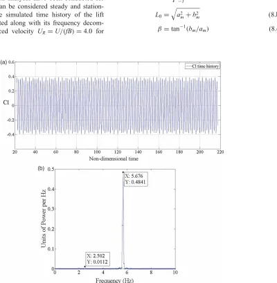
The main components of the unsteady wind force act-ing on the oscillatact-ing bluff-body are the vortex-sheddact-ing frequency component and the forced frequency compo-nent. In the results that are going to be presented below, the initial transient region in the simulations has been excluded and the data analyses have been conducted for time histories that can be considered steady and station-ary. In Figure 1 the simulated time history of the lift coefficient is presented along with its frequency decom-position for a reduced velocity UR=U/(fB)=4.0 for
the 4:1 rectangular cylinder (where f =ωm/2π the
fre-quency of oscillation in Hz). The first peak, at 2.5 Hz, corresponds to the frequency of oscillation while the sec-ond one, at 5.7 Hz, identifies the vortex shedding fre-quency. The component of the unsteady lift force (or moment) at the frequency of the forced oscillation can be written as:
Lm(t)=L0sin(ωmt+β) (7)
Where L0 is the amplitude of the unsteady lift at the
excitation frequency, andβ is the phase shift with respect to the forced oscillation.
Applying the Fourier decomposition of the unsteady lift force per unit of span length,L0andβcan be obtained:
[am, bm]=
1
T
T
∫
−T
L(t)[cosωmt, sinωmt]dt (8.a)
L0 =
a2
m+b2m (8.b)
β =tan−1(bm/am) (8.c)
(a)
[image:6.610.143.543.294.703.2](b)
Figure 1. Ratio 4:1 rectangular cylinder (a) time history and (b) spectral content of the lift coefficient at forced oscillation in the heave degree of freedom.
And the forced frequency component of the unsteady lift force acting on the bluff-body is:
Lm(t)=L0cosβsin(ωmt)+L0sinβ cos(ωmt) (9)
Where LmR=L0cosβ is the in-phase component and
LmI =L0sinβis the out-of-phase component of the forced
frequency term of the unsteady lift force. The out-of-phase component is of great importance since it plays the role of the aerodynamic damping, while the in-phase component plays the role of the aerodynamic stiffness. When the out-of-phase component is positive, it acts as negative aerody-namic damping indicating that self-excited oscillation may take place (see Shimada and Ishihara (2012) and Sarwar and Ishihara (2010), for a more detailed explanation).
The in-phase and out-of-phase components of the forced frequency component of the unsteady lift force can be expressed as nondimensional coefficients:
CLR=
LmR
1 2ρU2B
(10.a)
CLI =
LmI
1 2ρU2B
(10.b)
The same principles can be applied to the forced fre-quency component of the unsteady moment for the pitch degree of freedom. In this case, the nondimensional coeffi-cients are written as follows:
CMR=
MmR
1 2ρU2B2
(11.a)
CMI =
MmI
1 2ρU2B2
(11.b)
whereMmRis the in-phase component andMmIis the
out-of-phase terms of the forced frequency component of the unsteady moment.
5. Flutter derivatives computation by means of forced oscillation simulations
Flutter derivatives are nonanalytical parameters which relate motion-induced forces and the velocities and move-ments of the structure. As a consequence, these parameters have been traditionally identified using wind tunnel tests, and more recently from numerical-based simulations.
According to Sarkar, Caracoglia, Haan, Sato, and Murakoshi (2009) and Simiu and Scanlan (1996), the aeroelastic forces on a bridge deck, considering two degrees of freedom (heave and pitch) can be written as
follows, using Scanlan’s formulation: [
LSae(t)= 1
2ρU
2B
KH1∗h˙(t) U +KH
∗ 2
Bα(˙ t) U +K
2H∗ 3α(t)
+K2H4∗h(t) B
(12.a)
MaeS(t)= 1
2ρU
2B2
KA∗1h˙(t) U +KA
∗ 2
Bα(˙ t) U +K
2A∗ 3α(t)+
K2A∗4h(t) B
(12.b)
WhereLS
ae(t)is the aeroelastic lift force per unit of span
length,MS
ae(t)is the aeroelastic moment per unit of span
length,K=(Bω)/U is the reduced frequency, h(t)is the heave oscillation and h˙(t) is its time derivative, α(t) in the torsional rotation andα(˙ t)its time derivative,Hi∗ and
A∗i(i=1,. . ., 4) are the flutter derivatives.
Assuming prescribed harmonic forced oscillationsh= h0sin(ωht) and α=α0sin(ωαt), where h0 and α0 are
the amplitudes of the oscillations, and also that motion-induced forces are linear functions of the movement; after some manipulation, the following expressions are obtained for the identification of the flutter derivatives:
H1∗= −L0sinφL
qK2h0 (13.a)
H2∗= −L0sinφL qBK2α
0
(13.b)
H3∗= L0cosφL qBK2α
0
(13.c)
H4∗= L0cosφL qK2h
0
(13.d)
A∗1= −M0sinφM
qBK2h0 (13.e)
A∗2= −M0sinφM qB2K2α
0
(13.f)
A∗3= M0cosφM qB2K2α
0
(13.g)
A∗4= M0cosφM
qBK2h0 (13.h)
WhereL0andM0are the amplitudes of the fluctuating lift and moment acting on the bluff-body,φL andφM are the
phase lags of the aeroelastic lift or moment with respect to the prescribed oscillation andqis the dynamic pressure.
The adopted sign criterion has been the one reported in Sarkar et al. (2009) that is aeroelastic lift force and heave displacement positive downwards, moment and pitch rota-tion positive in the clock-wise direcrota-tion, for a flow coming from the left side.
The aerodynamic force representation employed by Washizu and co-workers (Washizu, Ohya, Otsuki, & Fujii,
1978;1980) is equivalent to the flutter derivatives formu-lation proposed by Scanlan. In this respect, in Sarkar et al. (2009), the expressions relating the out-of-phase and in-phase components of the lift and moment coefficients with the direct flutter derivativesH1∗,H4∗,A∗2andA∗3are derived.
6. Geometry and computer modeling
As it has been previously noted, a rectangular section with a width to depth ratioB/H =4 and sharp edges has been chosen as the case study for computing its forced oscillation response.
In the FSI simulations the rectangular cylinder, which is considered as rigid, is forced to oscillate at a prescribed frequency in heave or pitch degrees of freedom. In the adopted approach no structural solver is involved and the mesh movement is handled by the solver using the ALE method.
6.1. Boundary conditions
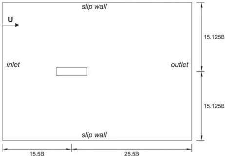
The flow domain size adopted in all the simulation reported herein is 41B by 30.25B, similar to the size employed in successful simulations by other researchers (Bruno, Fran-sos, Coste, & Bosco,2010; Fransos & Bruno,2010) and bigger than flow domains in Sun et al. (2008), Sarwar and Ishihara (2010) or Arslan, Pettersen, and Andersson (2011). The flow domain size has been chosen in order to guarantee that flow conditions near the bluff body are not influenced by the distance to the boundaries.
[image:8.610.60.291.545.705.2]As boundary conditions, a constant velocity inlet has been set at the left side (see Figure2) while a pressure out-let at atmospheric pressure has been imposed at the right side. The upper and lower boundaries have been defined as slip walls, that is, neglecting viscous effects caused by the wall surface. Taking into account that in the region close to these boundaries the flow is practically undisturbed, given the distance of the upper and lower boundaries from the
Figure 2. Flow domain definition and boundary conditions (rectangular cylinder out of scale).
bluff body, this is similar to imposing the uniform value of the inlet velocity along these boundaries as in Fransos and Bruno (2010) or Sarwar and Ishihara (2010). The walls of the rectangular cylinder surface are modeled as no-slip, taking into account that in the forced oscillation simula-tions the kinematic requirement that no flow can cross the wall is enforced (Donea, Huerta, Ponthot, & Rodríguez-Ferrán, 2004). In the solver, the resultant velocity field around the rectangular cylinder wall is corrected, impos-ing that the velocity at the boundary is equal to the mesh velocity and therefore no flux across the wall takes place.
A turbulence intensity of 1% has been chosen along with a 0.1B turbulent length scale for the incoming flow, as in Ribeiro (2011). This has the same order of magnitude as the 3% turbulence intensity and 0.082B turbulent length scale values in Sarkic et al. (2012).
A 2D block structured regular mesh has been gener-ated taking special care in the definition of the refined grid around the deck cross-section in order to obtain tar-get values for the nondimensional first grid height(y+=
(δ1u∗)/ν, whereδ1 is the height of the first prismatic grid
layer around the deck andu∗is the friction velocity) close to 1. In this manner, no wall functions are required.
The forced oscillation simulations have been conducted using a transient solver for incompressible flow of Newto-nian fluids on a moving mesh by means of the PIMPLE (merged PISO-SIMPLE) algorithm distributed with Open-FOAM (2014a). The interpolation of values from the cell centers to face centers is done using a linear scheme and the gradient terms are discretized using the cell limited version of the Gauss discretization scheme. In the same manner, the divergence terms are discretized by means of the Gauss schemes. For the Laplacian terms, the Gauss scheme with a linear interpolation scheme for the diffusion coefficient and a limited surface normal gradient scheme has been chosen. The first-order time derivative is dis-cretized using the Euler implicit scheme. Concerning the temporal discretization, the PISO scheme discretizes the momentum equations in an implicit manner, while the pres-sure gradient is explicit (OpenFOAM,2014b,2014c). The segregated operator splitting in PISO results in a solu-tion that is highly sensitive to Courant number, although certain aspects of the discretization are implicit. Thus, Courant numbers below 1 are generally required to main-tain stability.
6.2. Mesh control
The computer implementation of the ALE formulation requires a mesh-update method that assigns mesh-node velocities or displacements at each calculation time step (Donea et al.,2004). The computational grid must be kept as regular as possible, avoiding distortions and the squeez-ing of mesh elements, and therefore decreassqueez-ing numerical errors.
In the fluid structure interaction simulations conducted in this piece of research the boundary motion is defined by the prescribed forced oscillations of the rectangular cylin-der, which follows a sinusoidal law with given frequency and amplitude. On the other hand, the exterior boundaries of the fluid domain are fixed along the simulations.
Amongst the available mesh movement algorithms a Laplacian smoothing technique for each component of the node-mesh position has been chosen (Oliver, 2009). According to Jasak and Rusche (2009), the Laplace equation can be expressed as:
∇ ·k∇u=0 (14)
whereuis the node-mesh displacement vector and k is the diffusion coefficient.
In this work the diffusivity of the field is computed based on the quadratic inverse distance from the oscillat-ing boundary. This prevents the distortion of the smallest elements around the rectangular cylinder (Löhner,2008).
6.3. Verification studies
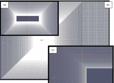
A grid independence study has been conducted for three different grids, namely Coarse, Medium and Fine grids, for the static rectangular cylinder with 0° angle of inci-dence. The thickness of the high-density layer attached to the rectangular cylinder is B/8. The mesh comprises 80 rows of elements in this zone and the height of the first element around the cross-section is the same for the three meshes considered in the verification study, and is defined as δ1/B=2.44×10−4. Besides this, the expansion
fac-tor (ratio between the dimension of the furthest and the closest elements to the wall) is 20. As a consequence, the mean value ofy+around the rectangular cylinder is about 0.9–0.95 and a maximum value, limited to the windward corners, is approximately 5.25, well below the maximum value of 8 reported in Sarkic et al. (2012) for a streamlined deck cross-section (see Figure3for images of the Medium grid). The Reynolds number of the simulations reported herein isRe=(UB)/ν=1.06×105 In Table 1 the data
(a) (b)
[image:9.610.116.498.332.609.2](c)
Figure 3. Block-structured grid: (a) close-up of the rectangular cylinder; (b) a larger region around the cylinder and (c) detail around the corner.
Table 1. Properties and results of the grid-refinement study.
Grid Total cells Cells around body St CD CD CL CM
Coarse 104000 560 0.145 0.31 0.009 0.27 0.046 Medium 147600 680 0.145 0.31 0.012 0.28 0.046 Fine 235200 880 0.145 0.31 0.011 0.29 0.045
[image:9.610.141.471.671.731.2]Table 2. Results of the time-refinement study.
Max. Co.
numb. s St CD CD CL CM
1 3.e-4 0.145 0.31 0.012 0.28 0.046 0.5 1.5e-4 0.143 0.31 0.013 0.28 0.047
of these three grids, along with the Strouhal number and the mean values and standard deviations of the force coeffi-cients are reported. All the computations have been carried out imposing a maximum Courant number of 1.
The definition of the force coefficients in this work is the following:
CD=
D 1 2ρU2B
CL=
L 1 2ρU2B
CM =
M 1 2ρU2B2
(15)
In the former expressions,Dis the drag force per span length, positive windward, L is the lift force per span length, positive upwards, andM is the twist moment per unit of span length, positive in the clock-wise direction. The reference dimension for the three coefficients is B. The standard deviation of the force coefficients is identified with the prime symbol in the following.
Table 1shows very similar results for the three grids considered, which highlights the level of independence of the solution from the mesh density. For the simula-tions hereafter the Medium grid has been retained since it offers similar accuracy to the Fine mesh with lower com-putational cost and its extra spatial resolution with respect to the Coarse mesh offers additional guaranties for the more demanding fluid-structure interaction simulations to be addressed in the present research.
Two different maximum Courant numbers have been considered for studying the stability of the numerical sim-ulation depending on the time step discretization: 1 and 0.5. The corresponding mean nondimensional time-steps, have been: s=(tU)/B≈3.0×10−4and 1.5×10⁻⁴.
[image:10.610.321.550.91.221.2]In Table2 the results obtained for the Medium mesh are reported. It has been found that both maximum Courant numbers offer very similar results, thus the higher has been retained hereafter.
Table 3. B/H = 4 rectangular cylinder: results and valida-tion.
St CD CD CL CM
Present simulation 0.145 0.31 0.012 0.28 0.046 Sun et al. (2009)
-2D URANS
0.15 0.33 0.024 0.351 0.053
Vairo (2003) - 2D URANS
0.149 0.356 0.065 0.25 0.071
Okajima (1982); Nakaguchi et al. (1968) - EXP.
0.135 0.30
Vairo (2003) - EXP. by CSTB
0.159 0.348 0.081 0.289 0.054
In the simulations which are going to be presented next, the nondimensional time steps are roughly between 3.0× 10⁻⁴and 2.5×10⁻⁴.
The FSI problems have been solved in a High Perfor-mance Computer Cluster which mainly comprises nodes with 2 AMD 8 cores processors. The forced oscillations in pitch simulations have been computed in parallel using 8 cores for each simulation. The heave-related problems, which demanded lower computational power, were solved using 4 cores in parallel. The execution time per time step has been about 4.5 seconds, depending obviously on the specific node load during the simulation.
7. Results and discussion
7.1. Flow simulation around the static rectangular cylinder
In Figure4the time history of the force coefficients for the static ratio 4:1 rectangular cylinder can be seen.
As a first step in the validation of the computa-tional results reported in this work, the main aerodynamic integral parameters are presented and compared with avail-able experimental and numerical results in the literature. The Strouhal number is computed from the dominant fre-quency in the spectrum of the lift coefficient. In Table 3
[image:10.610.124.483.588.715.2]the aforementioned results are summarized along with the standard deviation of the force coefficients and compared
Figure 4. Time history of force coefficients for theB/H = 4 static rectangular cylinder.
with numerical and experimental results reported in the literature.
It has been found that both mean drag force coeffi-cient and the Strouhal number predicted in this study fall inside the range of the experimental data available in the literature. Also the results are similar to other numerical simulations carried out using a 2D URANS approach (Sun et al., 2009; Vairo, 2003). Some differences have been found in the standard deviation of the force coefficients with respect to both experimental and numerical publica-tions; in fact, Bruno and co-workers, have pointed out the existing scattering in the literature for standard deviation of the lift coefficient for rectangular cylinders with high aspect ratios (Bruno et al.,2010). It has been found that the results obtained in this work for the standard deviation of the lift and moment coefficients are very close to the exper-imental values reported in Vairo (2003), while the standard deviation of the drag coefficient is lower, although all the available results collected agree in pointing towards a low value for the standard deviation of the drag coefficient, well below 0.1.
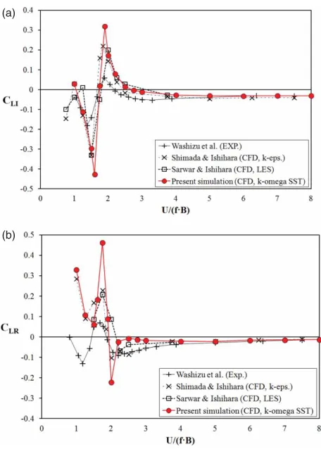
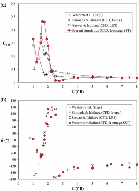
7.2. One degree of freedom heave forced oscillation With the aim of exploring the feasibility of the 2D URANS approach using Menter’s SST k-ω turbulence model in fluid-structure interaction problems, the forced oscillation response of the B/H = 4 rectangular cylinder has been computed. The amplitude of the oscillation ish0/D=0.02 as in the experimental tests conducted by Washizu et al. (1978). These forced oscillation simulations with constant flow speed and at different frequencies allow the identifica-tion of the reduced velocity regions where vortex-induced vibration can take place (Sarwar & Ishihara, 2010). The change in the out-of-phase component of the unsteady lift force from negative to positive values indicates that vortex-induced vibrations will occur due to the negative aerodynamic damping introduced in the system for positive values ofCLI.
The current numerical results are compared with the experimental ones in the former reference by Washizu and co-workers, along with the computational results reported in Sarwar and Ishihara (2010) and Shimada and Ishi-hara (2012). In the first reference concerning CFD, a 3D approach with a LES turbulence model is employed; while in the latter one, the authors successfully applied a 2D URANS approach using a two-layerk-ε turbulence model modified in the production term. In Figures 5(a) and 5(b) the out-of-phase and in-phase components of the lift coefficient are reported. Also, in Figures6(a) and 6(b) the amplitude of the unsteady lift coefficient at the fre-quency of oscillation and the phase difference between the forced displacement in the heave degree of freedom and the forced oscillation component of the lift force are shown. It must be noted that in Sarwar and Ishihara (2010) and Shimada and Ishihara (2012) the values ofCLRandCL0are
(a)
[image:11.610.319.547.62.381.2](b)
Figure 5. B/H = 4 rectangular cylinder lift coefficient (a) Out-of-phase component; (b) In-phase component.
not reported, however they have been computed for this study from the availableCLI andβ data in order to
pro-vide the complete picture in Figures5(b) and 6(a). From a qualitative perspective, the CFD results obtained in the frame of the current study agree well with the experimental data reported by Washizu et al. (1978): a region show-ing positive values of the out-of-phase component (CLI)
has been identified and the phase difference between the forced displacement and the forced oscillation component of the lift coefficient, for different reduced velocities, has also been obtained. However, a closer look at these results allows a further understanding of the turbulence model performance. As it has already been mentioned, the out-of-phase component of the lift coefficient is of utmost impor-tance since it allows the identification of reduced velocity regions prone to VIV. From Figure 5(a), the V-shaped branch in the range of reduced velocities (1.0, 1.7) has been captured as well as the inverted V-shaped branch between reduced velocities (1.7, 2.5). In the same manner, a curved branch in the interval (2.5, 4.0) and the nearly hor-izontal branch in the range (4.0, 8.0) have been correctly identified. Nevertheless, differences between the numerical values in the CFD simulations and the experimental tests are apparent. In fact the numerical simulations reported herein overestimate the magnitude of the peak of the V-shaped branch at UR=1.6. Also the peak in the inverted
(a)
[image:12.610.60.293.63.383.2](b)
Figure 6. B/H = 4 rectangular cylinder lift coefficient (a) Amplitude of the forced frequency component of the lift coef-ficient; (b) Phase angle.
V-shaped branch for UR = 1.9 is significantly higher
than the experimental value in Washizu et al. (1978) (see Table4).
These discrepancies can be explained as follows: The simulations have been obtained by means of 2D URANS simulations, therefore the predicted force coefficients show unrealistic smooth and periodic oscillations (Mannini et al.,
2010b) since complex turbulence phenomena are not resolved. Furthermore, in Brusiani, de Miranda, Patruno,
Ubertini, and Vaona (2013) it is noted that for RANS mod-els based on the Boussinesq hypothesis, 2D simulations are equivalent to 3D simulations showing perfect correlation in the span-wise direction. As a consequence, the aerody-namic forces are generally overestimated. Consequently, in this simulation, the forced frequency component of the lift force is expected to be higher than in the physical experiments. At reduced velocities equal to 1.6 and 1.9 the frequency of vortex shedding is locked-in with the frequency of oscillation, therefore the out-of-phase com-ponent of the lift coefficient is strongly over-predicted. The same phenomenon takes place at reduced velocities of 1.75 and 2.0, which are the peaks in the in-phase component of the lift coefficient chart (see Figure 5(b). In the same manner, Figure 6(a) shows high values for the amplitude of the forced frequency component of the lift coefficient in the range of reduced velocities (1.5, 2.0), and these val-ues are higher than in the other CFD-based references used for comparison.
Also a region of reduced velocities between 2.2 and 3.0 can be indentified which corresponds to the range of frequencies of oscillation below the frequency of vor-tex shedding and therefore this is the region where the lock-in must be surpassed. It has been found that the SST k-ω model has not been able to properly simulate this complex FSI region. This problem manifests itself in the underestimation of the in-phase component of the lift coefficient in that range of reduced frequencies, and the extension of the range of reduced velocities showing positive values for the out-of-phase component. Simi-lar behavior can be identified in the amplitude CL0 (see
Figure6a).
Furthermore, the phase difference between the forced oscillation lift force component and the heave forced dis-placements has not been correctly obtained for UR= 2.2
and UR=2.5 (see Figure6b) which corresponds to phase
[image:12.610.60.550.606.731.2]angles close to 180° according to Washizu et al. (1978). On the other hand, the turbulence model has offered results very close to the experimental ones in the range of reduced velocities (4.0, 8.0), which corresponds to the region where the complex VIV aerodynamic response has
Table 4. Discrepancies in the definition of the out-of-phase component of the forced frequency component of the lift coefficient using different turbulence models.
EXP. (Washizu et al., 1978)
k-ε(Shimada & Ishihara,2012)
LES (Sarwar &
Ishihara,2010) SSTk-ω
CmaxLI 0.06 0.22 0.2 0.3183
CminLI −0.18 −0.33 −0.33 −0.4274
RangepositiveCLI 1.765, 2.05 1.75, 2.25 2, 2.5 1.75, 2.5
U+R 0.285 0.5 0.5 0.75
e(CmaxLI ) 2.67 2.33 4.30
e(CminLI ) 0.83 0.83 1.37
e(U+R) 0.75 0.75 1.63
been overcome. Similar issues can be identified, with lower severity, in Shimada and Ishihara (2012) and Sarwar and Ishihara (2010).
With the purpose of assessing the level of accuracy offered by the SSTk-ωturbulence model and thek-εand LES models, the main features in the definition of the out-line of the CLI component are compared with the wind
tunnel data in Table 4. The following magnitudes have been considered: the maximum and minimum values of the out-of-phase component of the forced frequency term of the lift coefficientCmaxLI andCminLI ; the range of reduced velocities with positive values of CLI and the length of
the corresponding interval U+R. The discrepancies are estimated as:
e= |exp.value−num.value|
|exp.value| (16)
It must be borne in mind that the number of reduced frequencies considered in the numerical simulations and the experimental tests are different, as they are also differ-ent the concrete values of the reduced velocities adopted in each work. Therefore the values reported in Table 4
must be considered as an approximation for the purpose of assessing the accuracy of the different models.
According to the data reported in Table 4, it can be concluded that in spite of the qualitative agreement of the SSTk-ωturbulence model with the experimental data, its accuracy is lower than the k-ε and LES models, since it predicts higher peaks in theCLI and the range of reduced
frequencies showing positive values inCLIis also
overesti-mated (for practical applications this is in the safe side). It is remarkable the performance of the 2Dk-εmodel which at least matches the 3D LES results. In this respect, the lower overestimation of the peak values when compared with the SSTk-ωmodel can be related with the behavior of the modifiedk-εmodel, since in Shimada and Ishihara (2002) it is noted that the fluctuations in the lift force were considerably underestimated in some cases, as the 4:1 ratio rectangular cylinder.
In the above discussion the range of reduced velocities (4.0, 8.0) has not been considered since it is outside the VIV prone region, no significant discrepancies have been observed and that range will be specifically considered in the latter discussion on the flutter derivatives estimation.
7.3. One degree of freedom pitch forced oscillation The engineering interest in analyzing the response of a bluff-body undergoing harmonic torsional oscillation under wind flow lies in identifying the possibility of tor-sional flutter taking place at a certain range of reduced velocities, when the out-of-phase component of the moment coefficient changes from negative to positive values.
For the B/H = 4 rectangular cylinder, the amplitude of the pitch oscillation in the current simulations has been
α0=3.82◦, as in the experiments reported in Washizu et al.
(1980) and the numerical simulation in Shimada and Ishi-hara (2012). In Figure 7.a and 7.b the out-of-phase and in-phase components of the unsteady moment (CMI and
CMR) are reported along with equivalent experimental and
numerical results for validation.
The plot of the out-of-phase component of the moment coefficient as a function of the reduced velocity is qualitatively similar to the experimental values. The positive values of the out-of-phase component allow iden-tifying the range of reduced velocities for which the cross-section is prone to torsional flutter. In the CFD simulation the reduced velocity for whichCMI is null is lower than in
the wind tunnel tests, which is in the safe side for design applications. When the current simulation is compared with the one reported by Shimada and Ishihara, it can be concluded that the overall behavior is similar: both of them are shifted upwards in the vertical axis fromUR=3.0, but
without great differences with respect to the wind tunnel experiments.
For the sake of completeness, the amplitude of the forced frequency component of the moment coefficient and the phase angle with the forced oscillation in pitch degree
(a)
[image:13.610.320.549.378.708.2](b)
Figure 7. B/H = 4 rectangular cylinder moment coefficient (a) Out-of-phase component; (b) In-phase component.
of freedom are reported in Figures8(a) and 8(b). The data labeled as Shimada and Ishihara (CFD, k-eps.) have been computed from theCMRandCMI data reported in Shimada
and Ishihara (2012).
In this case, since the changes in the out-of-phase component of the forced frequency moment coefficient
CMI with the reduced velocity are smooth, an order
two polynomial can be approximated (see Figure7a) for the experimental values as well as the numerical values reported in the present work and in Shimada and Ishihara (2012). This allows the level of accuracy in the 2D URANS simulations to be judged when compared with the wind tunnel data. In order to provide a global assessment for the range of reduced velocities studied, the error is estimated
(a)
[image:14.610.61.292.262.582.2](b)
Figure 8. B/H = 4 rectangular cylinder moment coefficient (a) Amplitude of the forced frequency component of the moment coefficient; (b) Phase angle.
Table 5. Discrepancies in the definition of the out-of-phase and in-phase components of the forced frequency component of the moment coefficient using different turbulence models.
k-ε(Shimada &
Ishihara,2012) SSTk-ω
e(CMI) 0.51 0.59
e(CMR) 0.27 0.33
from the following expression:
e=∫
UfR
U0
R|
exp.aprox.−num.aprox.|dUR
∫UfR
U0
R|
exp.aprox|dUR
(17)
Where exp. aprox. and num. aprox. are the order two polynomial approximations for the experimental and numerical data; and U0
R and U f
R are the bounds of the
considered interval.
In Table 5 the reported results for the out-of-phase component correspond to the interval of reduced velocities (1.75, 8.0), which is the one for which the results are avail-able for the experimental test and the CFD simulations. It can be concluded that the SSTk-ωoffers slightly poorer accuracy when compared with the modifiedk-εmodel in Shimada and Ishihara (2012).
Furthermore, the results for the in-phase component
CMR show a similar trend as in Shimada and Ishihara’s
paper, with overestimated values atUR<3.5, but
particu-larly for reduced velocities in the interval (1.0, 2.0). In the former reference it is argued that this phenomenon, which was found also for rectangular cylinders of ratio 2:1 and 5:1, could be linked with the lack of turbulence diffusion in 2D models.
On the other hand, for reduced velocities above 3.5, both turbulence models offer results very close to the experimental ones. In this case a polynomial of order 4 has been approximated for the experimental data since it offers a very close match with the available points. The accuracy of the different numerical approaches is assessed using the expression in Equation (17) and the results are also pre-sented in Table5. The range of reduced velocities has been
U0
R =1.75 andU f
R =8.0. In this case also, the modifiedε
turbulence model has provided slightly better results than the SSTk-ωmodel.
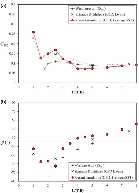
7.4. Flutter derivatives computation
The flutter derivatives of the B/H=4 rectangular cylin-der have been computed from the same forced oscillation simulations in heave and pitch degrees of freedom that have been employed to obtain the VIV and torsional flutter response presented in previous sections. In this way, always costly simulations have been avoided, which enhances the feasibility and industrial applicability of the computational-based approach proposed.
A VIV prone region around UR=2 was identified in
section6.2. Therefore for the heave-related flutter deriva-tives H1∗,H4∗,A∗1 and A∗4 the range of reduced velocities considered is (2.5, 8.0), while for the pitch-relatedH2∗, H3∗,
A∗2and A∗3flutter derivatives the range of reduced velocities is (2.0, 8.0).
In Figure 9 the numerical results are presented along with the experimental data in Matsumoto, Yagi, Tamaki,
[image:14.610.69.288.671.727.2]Figure 9. Flutter derivatives of theB/H = 4 rectangular cylinder: numerical results and comparison with experimental and numerical data.
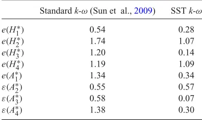
Table 6. Discrepancies in the flutter derivatives for the 4:1 rectangular cylinder computed from the stan-dard and the SST versions of thek-ωmodel.
Standardk-ω(Sun et al.,2009) SSTk-ω
e(H1∗) 0.54 0.28
e(H2∗) 1.74 1.07
e(H3∗) 1.20 0.14
e(H4∗) 1.19 1.09
e(A∗1) 1.34 0.34
ε(A∗2) 0.55 0.57
ε(A∗3) 0.58 0.07
ε(A∗4) 1.38 0.30
and Tsubota (2008) and the computational ones reported in Sun et al. (2009). Second-order polynomial approxima-tions are also included, which allow judging the general agreement between numerical simulations and wind tun-nel tests, and assessing the accuracy of the numerical approach.
The comparison of the reported results with the wind tunnel test data show, in general terms, that they are very similar. In fact the only remarkable differences take place for theH2∗andH4∗ flutter derivatives at reduced velocities above 4. On the other hand flutter derivativesH3∗orA∗3are extremely close to the experimental data.
A better general agreement for the current computa-tions has been found than the numerical simulacomputa-tions in smooth flow in Sun et al. (2009). This is arguably due to the higher size of the flow domain which prevents blockage effects and the higher mesh density adopted in the current work. Also the block structured mesh must play a role in the improved results since unstructured meshes are more diffusive, as it has been noted in Mannini et al. (2010a). Furthermore, Menter’s SSTk-ωturbulence model seems to offer better performance than the standardk-ωemployed by Sun and co-workers.
In Table 6 the accuracy of the numerical simulations with respect to the experimental data in Matsumoto et al. (2008) is assessed base on the second-order polynomial approximations. The error is estimated (Equation 17) in the range of reduced velocities (0, 8.0), except for the flut-ter derivatives H2∗ and H4∗, where the reduced velocities considered are between 0 and 6.0 since the discrepan-cies are important above the latest value, and the max-imum reduced velocity considered in Matsumoto et al. (2008) is 5.30. It can be remarked that in this case the SST k-ω model offers a remarkable agreement with the experimental data. In fact it has offered a better approx-imation for all the flutter derivatives considered in this work, with the exception of A∗2, when compared with the standardk-ωturbulence model employed by Sun and co-workers.
8. Concluding remarks
In this work a 2D URANS approach using a block-structured mesh and Menter’s SST k-ω turbulence model has been applied to the study of the fluid-structure interac-tion of a B/H = 4 rectangular cylinder. The aeroelastic phenomena of interest have been VIV, torsional flutter and the computation of flutter derivatives. A single set of heave and pitch forced oscillations has been considered for computing the responses of interest.
A study considering different mesh densities and time steps has been carried out, which has allowed guarantee-ing the stability of the solution in terms of grid and time step refinement as well as identifying the most convenient mesh and time step in terms of better accuracy at lower computational cost. The results obtained for the fixed rect-angular cylinder have been similar to the experimental ones available in the literature.
The SST k-ω turbulence model has been capable of identifying the region with positive values of the out-of-phase term of the forced frequency component of the lift coefficient as well as the phase difference between the forced heave displacement and the force frequency com-ponent of the lift force. As a consequence, the possibilities of the current approach, in the frame of industrial appli-cations where the preliminary identification of VIV prone regions is the main goal, have been demonstrated. When the obtained results are compared with the ones com-puted by Shimada and Ishihara by means of a modified
k-ε model, it is found that the SST k-ω models offers lower accuracy in the evaluation of the magnitude of the peak values or the extend of the region with positive values ofCLI.
In a similar fashion, the SSTk-ωmodel has correctly predicted the torsional flutter prone region for the 4:1 rectangular cylinder. However, when the results are com-pared with the modifiedk-εmodel in Shimada and Ishihara (2012), again the SSTk-ωmodel has offered slightly lower accuracy.
Where the SSTk-ωmodel offers a better performance is in the computation of the flutter derivatives. The agreement with the wind tunnel tests reported in Matsumoto et al. (2008) is remarkable. In this respect, the SST version offers higher accuracy than the standardk-ωturbulence model.
The current approach has proved its feasibility for identifying fluid-structure interaction responses, avoiding burdensome 3D LES simulations or the development of in-house sophisticated software. Therefore it is ready for being applied in the frame of parametric studies of bridge deck sections and, in the future, in the shape optimization of bridge deck considering aeroelastic constraints.
Acknowledgements
This work has been funded by the Spanish Ministry of Education, Culture and Sport under the Human Resources National Mobility Program of the R-D+i National Program 2008–2011, extended
by agreement of the Cabinet Council on October 7th 2011. It has also been partially financed by the Galician Government (includ-ing FEDER fund(includ-ing) with reference GRC2013-056 and by the Spanish Minister of Economy and Competitiveness (MINECO) with reference BIA2013-41965-P. The authors fully acknowledge the received support.
The authors are grateful for access to the University of Not-tingham High Performance Computing Facility and the Breogán Cluster at the University of La Coruña.
References
Arslan, T., Pettersen, B., & Andersson, H. I. (2011, July 10–15). Calculations of the flow around rectangular shaped floating structures. Proceedings of the 13th International Conference on Wind Engineering, Amsterdam, The Netherlands. Bai, Y., Sun, D., & Lin, J. (2010). Three dimensional numerical
simulations of long-span bridge aerodynamics using block-iterative coupling and DES.Computers and Fluids,39(9), 1549–1561.
Blazek, J. (2005).Computational fluid dynamics: Principles and applications(2nd ed.). Amsterdam: Elsevier.
Braun, A. L., & Awruch, A. M. (2003). Numerical simulation of the wind action on a long-span bridge deck.Journal of the Brazilian Society of Mechanical Sciences and Engineering, 25(4), 352–363.
Bruno, L., Coste, N., & Fransos, D. (2012). Simulated flow around a rectangular 5:1 cylinder: Spanwise discretisation effects and emerging flow features.Journal of Wind Engi-neering and Industrial Aerodynamics,104–106, 203–215. Bruno, L., Fransos, D., Coste, N., & Bosco, A. (2010). 3D
flow around a rectangular cylinder: A computational study. Journal of Wind Engineering and Industrial Aerodynamics, 98(6–7), 263–276.
Bruno, L., Salvetti, M. V., & Ricciardelli, F. (2014). Bench-mark on the aerodynamics of a rectangular 5:1 cylinder: An overview after the first four years of activity. Jour-nal of Wind Engineering and Industrial Aerodynamics,126, 87–106.
Brusiani, F., de Miranda, S., Patruno, L., Ubertini, F., & Vaona, P. (2013). On the evaluation of bridge deck flutter deriva-tives using RANS turbulence models. Journal of Wind Engineering and Industrial Aerodynamics,119, 39–47. Donea, J., Huerta, A., Ponthot, J. Ph., & Rodríguez-Ferrán,
A. (2004). Arbitray Lagrangian-Eulerian methods. Ency-clopedia of Computational Mechanics, Fundamentals, 1, 413–437.
Fransos, D., & Bruno, L. (2010). Edge degree-of-sharpness and free-stream turbulence scale effects on the aerodynamics of a bridge deck.Journal of Wind Engineering and Industrial Aerodynamics,98(10–11), 661–671.
Hernández, S., Nieto, F., Jurado, J. Á, & Pérez, I. (2012, Septem-ber 2–6). Bluff body aerodynamics of simplified bridge decks for aeroelastic optimization. Proceedings of the 7th International Colloquium on Bluff Body Aerodynamics and Applications, Shanghai, China.
Jasak, H., & Rusche, H. (2009, June 1–4). Dynamic mesh handling in OpenFOAM. Fourth OpenFOAM workshop, Montreal, Canada.
Kuroda, M., Tamura, T., & Suzuki, M. (2007). Applicability of LES to the turbulent wake of a rectangular cylinder – com-parison with PIV data.Journal of Wind Engineering and Industrial Aerodynamics,95(9–11), 1242–1258.
Le, T. H., Tamura, Y., & Matsumoto, M. (2011). Spanwise pressure coherence on prisms using wavelet transform and
spectral proper orthogonal decomposition based tools. Jour-nal of Wind Engineering and Industrial Aerodynamics, 99(4), 499–508.
Löhner, R. (2008).Applied computational fluid dynamics tech-niques: An introduction based on finite element methods (2nd ed). Chichester, UK: John Wiley.
Mannini, C., Soda, A., & Schewe, G. (2010a). Unsteady RAS modelling of flow past a rectangular cylinder: Investigation on Reynolds number effects.Computers and Fluids,39(9), 1609–1624.
Mannini, C., Soda, A., Voß, R., & Schewe, G. (2010b). Unsteady RANS simulations of flow around a bridge section.Journal of Wind Engineering and Industrial Aerodynamics,98(12), 742–753.
Mannini, C., Soda, A., & Schewe, G. (2011). Numerical investigation on the three-dimensional unsteady flow past a 5:1 rectangular cylinder. Journal of Wind Eng-ineering and Industrial Aerodynamics, 99(4), 469–482.
Matsumoto, M. (1996). Aerodynamic damping of prisms.Journal of Wind Engineering and Industrial Aerodynamics,59(2–3), 159–175.
Matsumoto, M., Yagi, T., Tamaki, H., & Tsubota, T. (2008). Vortex-induced vibration and its effect on torsional flut-ter instability in the case of B/D=4 rectangular cylinder. Journal of Wind Engineering and Industrial Aerodynamics, 96(6–7), 971–983.
Mendes, P. A., & Branco, F. A. (1999). Analysis of fluid-structure interaction by an arbitrary lagrangian-eulerian finite element formulation.International Journal for Numerical Methods in Fluids,30(7), 897–919.
Menter, F. R. (1994). Two-equation Eddy-viscosity turbulence models for engineering applications.AIAA Journal,32(8), 269–289.
Menter, F. R. (2009). Review of the shear-stress transport tur-bulence model experience from an industrial perspective. International Journal of Computational Fluid Dynamics, 23(4), 305–316.
Menter, F., & Esch, T. (2001, November 26–30). Elements of industrial heat transfer prediction. Proceedings of the 16th Brazilian Congress of Mechanical Engineering, Uberlandia, Brasil.
Murakami, S., Mochida, A., & Sakamoto, S. (1997). CFD analy-sis of wind-structure interaction for oscillating square cylin-ders.Journal of Wind Engineering and Industrial Aerody-namics,72, 33–46.
Nakaguchi, H., Hashimoto, K., & Muto, S. (1968). An experi-mental study on aerodynamic drag of rectangular cylinders. Journal of the Japan Society of Aeronautical and Space Sciences,16, 1–5.
Nieto, F., Kusano, I., Hernández, S., & Jurado, J. Á. (2010, May 23–27).CFD analysis of the vortex-shedding response of a twin-box deck cable-stayed bridge. Proceedings of the 5th International Symposium on Computational Wind Engineering, Chapel Hill, NC.
Norberg, C. (1993). Flow around rectangular cylinders: pressure forces and wake frequencies.Journal of Wind Engineering and Industrial Aerodynamics,49(1–3), 187–196.
Ogawa, K., Sakai, Y., & Sakai, F. (1988). Aerodynamic device for suppressing wind-induced vibration of rectangular section structures. Journal of Wind Engineering and Industrial Aerodynamics,28(1–3), 391–400.
Okajima, A. (1982). Strouhal numbers of rectangular cylinders. Journal of Fluid Mechanics,123, 379–398.
Oliver, A. (2009). Mesh motion alternatives in OpenFOAM. Project report: PhD course in CFD with OpenSource