The origin and dynamic interaction of solar magnetic fields

(1)

The origin and dynamic interaction of

solar magnetic fields

Antonia Wilmot-Smith

Thesis submitted for the degree of Doctor of Philosophy

of the University of St Andrews

(2)

Abstract

The dynamics of the solar corona are dominated by the magnetic field which creates its structure. The magnetic field in most of the corona is ‘frozen’ to the plasma very effectively. The exception is in small localised regions of intense current concentrations where the magnetic field can slip through the plasma and a restructuring of the magnetic field can occur. This process is known as magnetic reconnection and is believed to be responsible for a wide variety of phenomena in the corona, from the rapid energy release of solar flares to the heating of the high-temperature corona.

The coronal field itself is three-dimensional (3D), but much of our understanding of reconnection has been developed through two-dimensional (2D) models. This thesis describes several models for fully 3D reconnection, with both kinematic and fully dynamic models presented. The reconnective behaviour is shown to be fundamentally different in many respects from the 2D case. In addition a numerical experiment is described which examines the reconnection process in coronal magnetic flux tubes whose photospheric footpoints are spun, one type of motion observed to occur on the Sun.

The large-scale coronal field itself is thought to be generated by a magnetohydrodynamic dynamo op-erating in the solar interior. Although the dynamo effect itself is not usually associated with reconnection, since the essential element of the problem is to account for the presence of large-scale fields, reconnection is essential for the restructuring of the amplified small-scale flux. Here we examine some simple models of the solar-dynamo process, taking advantage of their simplicity to make a full exploration of their behaviour in a variety of parameter regimes. A wide variety of dynamic behaviour is found in each of the models, including aperiodic modulation of cyclic solutions and intermittency that strongly resembles the historic record of solar magnetic activity.

(3)

Declaration

I, Antonia Wilmot-Smith, hereby certify that this thesis, which is approximately 45,000 words in length, has been written by me, that it is the record of work carried out by me and that it has not been submitted in any previous application for a higher degree.

Signature of candidate . . . . Date . . . .

I was admitted as a research student in September, 2004 and as a candidate for the degree of Doctor of Philosophy in September, 2005; the higher study for which this is a record was carried out in the University of St Andrews between 2004 and 2007.

I hereby certify that the candidate has fulfilled the conditions of the Resolution and Regulations appropriate for the degree of Doctor of Philosophy in the University of St Andrews and that the candidate is qualified to submit this thesis in application for that degree.

Signature of supervisor . . . . Date . . . .

In submitting this thesis to the University of St Andrews I understand that I am giving permission for it to be made available for use in accordance with the regulations of the University Library for the time being in force, subject to any copyright vested in the work not being affected thereby. I also understand that the title and abstract will be published, and that a copy of the work may be made and supplied to any bona fide library or research worker.

(4)

Acknowledgements

I’d like to thank everyone who has helped out these past 3 years: Eric Priest, my supervisor, without whose encouragement I’d have never thought to begin this thesis and certainly would never have finished; Gunnar Hornig for considerable patience and so much of his time spent in persistently good humour; Ineke De Moortel for introducing me to the world of numerics with a likeminded attitude; Dibyendu Nandi for many entertaining discussions and Piet Martens, Klaus Galsgaard and Steve Tobias for collaborating on various chapters.

Finally, thanks are due to Montana State University for their hospitality and both them and the Particle Physics and Astronomy Research Council for financial support.

(5)

List of Figures

1.1 Solar eclipses – from solar maximum to minimum. . . 1

1.2 The sunspot cycle. . . 3

1.3 Basic mechanism of the stretch-twist-fold dynamo. . . 7

1.4 Sweet-Parker reconnection. . . 11

1.5 Petschek reconnection. . . 11

2.1 AR9373 observed by TRACE, 21/03/2001. . . 13

2.2 Structure of a 3D null-point. . . 17

2.3 Local/Global field configurations . . . 19

2.4 Contradiction of flux conservation . . . 20

2.5 Cartoon illustrating particular solution of Hornig and Priest (2003). . . 22

3.1 The magnetic fieldB0. . . 27

3.2 Non-ideal region in the case of constant current. . . 30

3.3 Non-ideal velocities in the case of constant current. . . 31

3.4 Snapshot from Pontin et al. (2005a) MHD experiment. . . 34

3.5 Pressure profile in particular solutions. . . 34

3.6 Contours ofA2. . . 36

3.7 Contours ofA0+M2 eA2. . . 37

3.8 Comparison of non-ideal regions. . . 38

3.9 Non-ideal velocities for non-constant current. . . 39

3.10 Ideal plasma velocity. . . 41

3.11 Composite pressure profile. . . 42

3.12 Flowswinandwout(I). . . 43

3.13 Flowswinandwout(II). . . 43

3.14 Flowswinandwout(III). . . 45

3.15 Accelerating stagnation flow. . . 47

3.16 Pressure profile and Lorentz force (I). . . 48

3.17 Current in the case of accelerating flow. . . 49

3.18 Pressure profile and Lorentz force (II). . . 50

4.1 GMR classification scheme. . . 54

(8)

4.2 Model for flux-tube disconnection. . . 56

4.3 Current expected in flux-tube disconnection. . . 56

4.4 Loop integral path. . . 57

4.5 Illustrative flux-tube. . . 60

4.6 3D localised current. . . 61

4.7 Counter-rotating foot-point motions. . . 62

5.1 Position and labels for magnetic flux sources. . . 71

5.2 Illustrative field-line evolution with spin-angle. . . 73

5.3 Flux connectivity of sourceA. . . 74

5.4 Change in magnetic flux connectivity with spin angle. . . 75

5.5 Flux connectivity in the central plane. . . 76

5.6 Contours of current in the central plane. . . 77

5.7 Variation of quantities across tangential discontinuity. . . 79

5.8 Current reversal at ends of non-ideal region. . . 80

5.9 Plasma flows in central plane. . . 80

5.10 Inflow gas and magnetic pressure. . . 81

5.11 Illustrative field lines and field topology. . . 82

5.12 Relation of field lines to contact discontinuity. . . 83

5.13 Complex flux connectivity in the central plane. . . 84

5.14 Comparison between aligned and misaligned sources. . . 84

6.1 Bifurcation curves and resonance tongues. . . 93

6.2 Parameterised path. . . 94

6.3 Magnetic activity after primary Hopf bifurcation. . . 95

6.4 Comparing frequency-locked and quasi-periodic solutions. . . 96

6.5 Poincar´e sections illustrating transition to chaos. . . 96

6.6 Chaotic solutions. . . 97

6.7 Solutions with an intermittent character (Ω = 11.023). . . 98

7.1 Cartoon illustrating solar cycle time-delay concept. . . 101

7.2 Quenching factor profile. . . 103

7.3 Example time-series for low-dynamo number in the flux transport dominated regime. . . . 108

7.4 Typical time-series in the flux transport dominated regime. . . 109

7.5 Dependence of cycle period and amplitude on dynamo number. . . 110

7.6 Dependence of cycle period and amplitude on time delay. . . 110

7.7 Typical time-series in the flux transport dominated regime – positive dynamo number. . . . 110

7.8 Typical time-series in the diffusion dominated regime. . . 113

7.9 Magnetic activity in diffusion dominated regime (I). . . 114

7.10 Magnetic activity in diffusion dominated regime (II). . . 114

7.11 Magnetic activity in diffusion dominated regime (III). . . 115

(9)

7.12 Magnetic activity in diffusion dominated regime (IV). . . 116

7.13 Mechamism for field reversal – diffusion dominated case. . . 118

7.14 Mechamism for field reversal – flux transport dominated case. . . 119

8.1 Exploring the effect of variable time-delaysT0. . . 124

(10)

Chapter 1

Introduction

Figure 1.1: The solar corona as observed during the total solar eclipses of (left) 1980, close to sunspot maximum, and (right) 1994, close to sunspot minimum. Source: High Altitude Observatory.

Plasmas do not form a significant part of our every-day environment and yet the stars, the interplanetary medium and the interstellar medium are all made of ionised gases. Indeed more than 99% of the visible matter in the universe consists of plasma. A physical understanding of these plasmas is, therefore, of major importance – but hard to come by since the huge spatial scales that characterise the problem are not available for realistic experiments on Earth. Instead, the natural laboratory to turn to is the solar corona, the outer atmosphere of the Sun.

The corona exhibits significant temporal and spatial variability (as has been observed in eclipses for centuries – see Figure 1.1). Its structure is created by the magnetic field that permeates it and is responsible for its extreme temperature; in the 1940s the corona was found to be several hundred times hotter than the underlying visible surface of the Sun, the photosphere. To understand the corona we must understand its magnetic field. Where does the field originate? How does it behave and what are the consequences of the behaviour? These are some of the questions we will examine in this thesis, but first we consider the structure of the Sun in more detail.

The Sun is estimated to have been luminous for about4.6×109years – the only energy source capable

(11)

2

of meeting such a long term requirement is nuclear fusion. The fusion process occurs in the core of the Sun, which extends to 20% of its radius, and is sufficiently hot 15×106_K_{and dense} ₁₅₀_g/cm−3 to sustain the reactions, the most important of which is the proton-proton reaction. Moving further away from the solar centre, the temperature and density decrease such that fusion stops, the transition marking the beginning of the radiative zone where energy is transported toward the surface by radiation. Photons travelling (net) outwards through the region continually undergo absorption and re-emission, so increasing their wavelength. When the temperature gradient required to transport the energy flux by radiation is larger than that of an adiabatically stratified hydrostatic equilibrium, the region becomes unstable to convection (the Schwartzschild criterion). As a result, convective fluid motions (which are very efficient in energy transport) occur in the outer 30% of the solar radius, which makes up the convection zone. As a source of mechanical energy they are ultimately responsible for the solar magnetic cycle and hence for the majority of solar dynamics. Large-scale convective motions are observed only indirectly, by their manifestations such as magnetic activity in the outer solar regions and the solar rotation profile (deduced by helioseismology), since they tend to be obscured by smaller-scale motions (such as granulation) close to the surface.

Helioseismology uses measurements of global acoustic oscillations on the solar surface (in visible light) to infer properties of the solar interior. Measuring frequency shifts in these p-mode (pressure-mode) os-cillations allows the internal velocity profile to be deduced. The convection zone is found to be rotating differentially, faster at the equator (P ≈25days) than the poles (P ≈35days) and, at mid-latitudes, the angular velocity contours are approximately radial. The radiative zone, however, rotates as a solid body, and there exists a sharp transition between the two rotational regimes. This transitional layer is known as the tachocline (Spiegel and Zahn, 1992, see Hughes et al. (2007) for a recent review) and estimates of its width vary from0.1% to0.9% of the solar radius, depending on how the tachocline is defined (for a discussion see Miesch, 2005). The rotation rate of the radiative zone lies between that of the polar region and the equatorial region of the convection zone and so a positive (negative) gradient in the radial angular velocity across the tachocline exists at low (high) latitudes

The radius of the Sun,RJ= 6.96×108m, is defined by its visible surface, the photosphere, where the

plasma becomes optically thin (as we move radially outwards). The photosphere is very thin, comprising only0.07% of the solar radius, and has a temperature of about5800K. The photosphere is the inner-most layer of the Sun that can be observed directly in great detail. Large-scale granulation and supergranulation patterns are seen, which, although associated with convection, are thought not to pervade the convection zone but to be confined to approximately only the outer 3% of the solar radius. Sunspots, regions of extremely intense field concentration, are another major photospheric feature. They are seen as small dark regions drifting across the surface as they are carried around by the rotating Sun. It was by tracking the motions of sunspots that the solar differential rotation was first inferred.

In the layer above the photosphere, known as the chromosphere, the temperature rises to around20000K. Emission inHαgives the chromosphere its distinctive red colour, as seen during solar eclipses in

promi-nences projecting above the limb. Promipromi-nences are regions where plasma at chromospheric temperatures

(12)

3

17000 1750 1800 1850 1900 1950 2000 20

40 60 80 100 120 140 160 180

year

international sunspot number

Figure 1.2: International Sunspot Numbers for the years1700−2005. The International Sunspot Number is given byR=K(10G+S)whereSdenotes the number of observed sunspots,Gthe number of observed sunspot groups and K a quality factor to allow for comparison of results from different observational locations. Data from 40–70 stations are used in the measurements and is compiled at the Royal Observatory of Belgium. Source: SIDC, RWC Belgium, World Data Centre for the Sunspot Index, Royal Observatory of

Belgium, 2007.

regions known as spicules – short lasting features in which plasma is ejected toward the corona. Other chromospheric features include plages and fibrils.

The transition region is a thin, highly irregular and dynamic layer that consists of plasma between chro-mospheric and coronal temperatures. Finally, the outer layer of the solar atmosphere is the solar corona. The dynamics of all coronal phenomena are controlled by the magnetic field. Although in coronal

seis-mology the first attempts are being made to measure the field directly using the properties of coronal waves

(Roberts et al., 1984), knowledge of the field is traditionally obtained by extrapolation from magnetograms at the photosphere (using potential or force-free models). The corona itself only becomes visible in white light when the solar disc is occulted – since it is very tenuous, its optical emission is several orders of magnitude less than that of the photosphere. It may, however, be observed in great detail in non-visible wavelengths (such as X-rays) because the brightest emission in these wavelengths comes from the corona and the photosphere is no longer visible.

The solar magnetic field exhibits dramatic spatial and temporal variability. Several of the changes are systematic and occur on very large-scales. For example, the number of sunspots on the face of the Sun varies in time in a cyclic but irregular manner (see Figure 1.2). The sunspot cycle varies in length but has an average period of approximately 11 years and, in addition, significant variations in cycle amplitude are present. As sunspots begin to emerge at the beginning of each cycle, they do so at (relatively) high latitudes of around27o_{degrees, but as the cycle progresses emergence tends to occur closer to the equator,}

up to around8o_{. Sunspots typically appear in pairs of opposite polarity, with the axis of a bipolar sunspot}

pair being tilted by about4o_{with respect to the equator (Joy’s law). The polarity of the leading sunspot}

(13)

1.1 The Equations of Magnetohydrodynamics 4

solar maximum where most of the corona is in the form of magnetically closed loops.

The coronal magnetic field is capable of storing huge amounts of energy as it is injected via turbulent photospheric motions. Its structure is observed to be continually changing on a wide variety of scales and a process known as magnetic reconnection is of fundamental importance in this respect. Reconnection is the only process that can change the magnetic field topology and is thought to be responsible for maintaining the unexpectedly high temperature of the corona as well as for a wide variety of explosive events such as

solar flares and coronal mass ejections (CMEs).

In the next section we introduce the equations needed to mathematically describe the behaviour of the solar magnetic field.

1.1 The Equations of Magnetohydrodynamics

In this thesis we will assume the magnetohydrodynamic (MHD) approximation. There are a number of conditions behind this assumption, as discussed in detail in, for example, Priest (1982), Boyd and Sanderson (2003). Briefly, MHD is a theory of non-relativistic macroscopic plasma phenomena. The plasma is treated as a single fluid, with the electron and ion species locked together and is considered quasi-neutral, so the charge density vanishes. Under the non-relativistic assumption the displacement current (that given by∂E/∂t/c2_{in Amp`ere’s law) can be neglected. By macroscopic we imply that the typical length- and} time-scales of interest are much larger than the typical microscopic length- and time-scales of the ion and electron dynamics (the ion Larmor radius and gyroperiod and the mean free path time and length).

The equations of MHD are:

Mass conservation

∂ρ

∂t +∇ ·(ρv) = 0, (1.1)

the equation of motion (or, momentum conservation)

ρDv

Dt =−∇p+j×B+F, (1.2)

the ideal gas law

p=ρRT , (1.3)

Amp`ere’s law

∇ ×B=µj, (1.4)

solenoidal constraint

(14)

1.1 The Equations of Magnetohydrodynamics 5

Faraday’s law

∂B

∂t =−∇ ×E, (1.6)

Ohm’s law

E+v_×B=R. (1.7)

These equations must also be supplemented by an appropriate energy equation. In the equationsBis the magnetic induction, normally referred to as the magnetic field,vis the plasma velocity,Ethe electric field,

jthe electric current density,ρthe mass density,pthe plasma pressure (assumed to be isotropic),_Rthe gas constant,T the plasma temperature,µthe magnetic permeability,Fdenotes other forces which may be present, such as that due to gravity. Note that if the solenoidal constraint holds at some timet = 0then, by taking the divergence of Faraday’s law, it remains valid for all timet > 0. The termRin Ohm’s law denotes a general non-ideal term. The basic assumption of resistive MHD is that the collisional effects in

Rare the dominant ones, with the resistivity normally considered the most important, i.e. R=j/σwhere σis the electrical conductivity.

It is common to combine (1.4), (1.6) and the resistive form of (1.7), to give the induction equation,

∂B

∂t =∇ ×(v×B) +η ′

∇2B (1.8)

whereη′ _{= 1}_/₍_µσ₎_{is the magnetic diffusivity. In this thesis we will frequently label}_η _{= 1}_{/σ, a} com-mon, and perhaps misleading, notation in the literature. In obtaining the induction equation, the magnetic diffusivity has been taken to be uniform. Generally, however, the conductivity is expected to vary in space through a dependence on the magnetic field and the plasma temperature. We will often take a spatially dependent conductivity in this thesis and so do not work directly from the induction equation, but use it here to infer important general properties of solar and astrophysical plasmas. If the termη′_∇2_B_{in (1.8)} is neglected we obtain the ideal induction equation which may be combined with the equation of mass continuity, (1.1), to give

D Dt

_B

ρ

=

_B

ρ

· ∇v.

The equation for the evolution of a material line element is

D

Dt(dl) =dl· ∇v,

and so we deduce that in the ideal limit the magnetic field lines move as if frozen into the plasma; this is Alfv´en’s theorem. If, however, the advective term_{∇ ×}(v_×B)is neglected, then the induction equation reduces to a purely diffusive equation.

The ratio of these two terms, in an order of magnitude sense, is termed the magnetic Reynolds number, Rmand is a measure of their relative importance:

Rm = |∇ ×(

(15)

1.2 The Need for a Solar Dynamo 6

= v0B0/l0

η′_B0/l2 0

= l0v0

η′ .

The magnetic Reynolds number is nearly always very large, particularly so in the solar (and astrophysical) case because of the huge spatial scales of the systems. Thus the magnetic field is almost always frozen-into the plasma and field topology is conserved, with important consequences for dynamics. Non-ideal terms may become important if the length scales associated with the problem are small, as is the case for example in thin current sheets. The magnetic field can then slip through the plasma, allowing for reconnection.

Another important dimensionless parameter to help characterise the behaviour of the plasma is the

plasma beta,β, which is the ratio of the gas pressure to the magnetic pressure:

β= 2µp0

B2 0 .

In the majority of the coronaβis very much less than unity, which has the effect of inhibiting cross-field transport. Accordingly plasma tends to flow from the chromosphere into the corona along magnetic field lines. Although there are exceptions – regions with very high temperature but low magnetic field may have valuesβ >1– most models of the coronal field essentially assumeβ ≪1.

1.2 The Need for a Solar Dynamo

Given the importance of the solar magnetic field in determining coronal dynamics it is natural to ask how the field originates. A frozen-in primordial field would decay in a time-scale of around109years, which is comparable to the age of the solar system. It is, however, very difficult to explain the large-scale temporal variability of the field (manifested for example in the sunspot cycle shown in Figure 1.2) as consistent with such a decay. Magnetic fields also are observed in a multitude of other astrophysical bodies. For example: our galaxy exhibits a large-scale field confined approximately to the plane of its disc (see, for example Han and Qiao, 1994, and references therein); very strong surface magnetic fields have been detected on many other stars (Preston, 1971, Landstreet, 1992, Baliunas et al., 1995); on the planetary scale the magnetic field of the Earth reverses polarity at apparently random intervals in time (e.g. Cox, 1969).

(16)

[image:16.595.110.494.97.458.2]

Figure 1.3: Cartoon illustrating the stretch-twist-fold sequence that demonstrates the possibility of expo-nential growth of the magnetic field. Stretching an incompressible closed flux tube to twice its original length reduces its cross section by half. Twisting and folding gives a tube with twice the flux and the same original cross section.

first example of a fast dynamo, one for which the growth rate of a magnetic field remains positive as the magnetic Reynolds number approaches infinity (with other dynamos being classed as slow). However, the model ignores dissipative effects, failing to take into account the strong field gradients that may arise in the process (particularly at large times) and allow diffusive effects to become important. In a more realistic dynamo model, the precise balance between driving and diffusion must be considered.

(17)

As discussed in Chapter 6, there have now been several advances in dynamo theory, beginning with Parker’s idea of anαΩ–dynamo operating in the solar convection zone (Parker, 1955). Although much of the work has side-stepped the difficulty of the nonlinear back-reaction on the flow by the Lorentz force by discussing only the kinematic problem (in which the flow is prescribed and the time variation of the magnetic field deduced) it has, nevertheless, shown that dynamos can work.

Parker (1955) suggested that non-axisymmetric small-scale helical convective motions could twist toroidal field into poloidal loops, with the net effect being the production of a large-scale poloidal field. This mechanism is classically known as the alpha effect although, both in this thesis and some of the liter-ature, the term is also used to denote any general toroidal to poloidal conversion mechanism. A significant step forward in the mathematical foundations of this theory came with the introduction of mean-field

elec-trodynamics (Steenbeck et al., 1966). Here the magnetic field, B, and flow, v, are written in terms of mean (B0(x, t),V0(x, t)) and fluctuating components (b0(x, t),v0(x, t)) where the mean fields vary on length-scales much larger than those of the fluctuating parts. An averaging procedure is taken over intermediate length-scales and so

B(x, t) =B0(x, t) +b(x, t), V(x, t) =V0(x, t) +v(x, t),

where_hv_i=hb_i= 0(if_h.idenotes averages). Under these conditions, the induction equation, (1.8), can be written in terms of mean and fluctuating parts, with the equation for the mean field being given by

∂B0

∂t =∇ ×(V0×B0) +∇ ×ε+η ′

∇2B0,

whereε = hv_×b_iis a mean electromotive force (e.m.f.) induced by the fluctuating components. The e.m.f. must then be expressed in terms of the mean fieldB0 so that closure of the system is obtained. A suitable relation, obtained by considering also the equation for the fluctuating field, the separation of scales and assuming the fluctuating flowvis isotropic, is given by

ε=αB0−β∇ ×B0,

which, in turn, gives the evolution equation for the mean field as

∂B0

∂t =∇ ×(V0×B0) +∇ ×αB0+ (η ′₊_β₎

∇2B0

We see thatβreflects a turbulent enhancement of the magnetic diffusivity andα(hence the ‘alpha effect’) parameterises a source-term for the mean field. If the fluctuating velocity field is not reflectionally sym-metric thenαwill be non-zero; this lack of reflectional symmetry is key for the development of dynamo action. In mean-field simulations bothαandβare given prescribed dependencies on the mean field withα typically falling-off in the presence of strong fields (this algebraicα-quenching represents the inefficiency of the alpha effect on strong magnetic fields). Mean-field theory has enjoyed much success in reproducing many of the observed large-scale solar magnetic features (such as the butterfy diagram) – for a review, for example, Hoyng (2003).

(18)

1.3 Magnetic Reconnection in Two Dimensions 9

such as the production of poloidal flux through the decay of bipolar active regions invoked in the Babcock-Leighton mechanism (Babcock, 1961, Babcock-Leighton, 1969). These models utilize the same poloidal to toroidal conversion mechanism as Parker’s approach but now the alpha-effect manifests itself as a surface phe-nomenon. Solar observations show that bipolar active regions appear on the photosphere with a systematic tilt (Joy’s law) and therefore have a net north-south dipole vector. In time the active regions decay or diffuse away and in the process the leading polarities migrate toward the equator whilst the trailing polarities move toward the poles. The opposite polarities that are transported equatorward from the Northern and Southern hemispheres cancel by the equator. Crucially, the polarities that move poleward act to replace the exist-ing poloidal field and reverse it sign. Thus the decay of bipolar active regions takes the role of a surface α-effect.

A brief discussion of the sign of the alpha-effect in these various models will also be helpful. Parker (1955) deduced that the sign of the product of αand the vertical differential rotation gradient must be negative in the northern hemisphere if the observed equatorward migration of active regions is to take place. This sign rule holds even if the differential rotation gradient and the alpha-effect are in different layers (Moffatt, 1978, Section 9.7). Through helioseismology the differential rotation gradient at low latitudes is known to be positive. In the framework of mean-field theory we expect a negative alpha-effect to act in the lower part of the convection zone. Cyclonic convection occurs throughout the convection zone. However, considering the observed differential rotation profile, if this type of dynamo action is to lead to the observed equatorward migration of active regions then we require a negative alpha effect in the Northern hemisphere. Such a negative alpha effect is believed to occur in the lower part of the convection zone only. In Babcock-Leighton models however, the alpha-effect is concentrated in the surface layers whereαmust be positive (since the trailing polarities of active regions are at higher latitudes on the photosphere than the following polarities). The problem of achieving an equatorward progagating dynamo wave is overcome by including a meridional flow with a short timescale in the model – and anyway Babcock-Leighton models must invoke such a flow for the transport of magnetic flux between the separated source layers.

It is likely to be some time before a full understanding of the dynamo process is reached – current analytical modelling tends to be based on somewhat tentative foundations, and numerical simulations far from being able to resolve the huge range of length- and time-scales inherent to the process. In this thesis (Chapters 6 and 7) we explore an alternative and complementary approach to traditional dynamo modelling and construct simple mathematical models that are expected to have a similar underlying structure to that of the full system. Their very simplicity allows us to fully explore their dynamics and so make inferences about the properties of both solar and stellar dynamos, while their physical justification is sufficiently general that they may be applied to a wide variety of the proposed dynamo mechanisms.

1.3 Magnetic Reconnection in Two Dimensions

(19)

plasma process that is responsible for a wide range of phenomena, being of importance in solar, space, astrophysical and laboratory plasmas, for example in:

• Heating the corona to its multi-million degree temperatures (e.g. Parker, 1983).

• Sudden violent events such as solar flares (Parker, 1963) and CMEs and the corresponding events on other stars.

• The Earth’s magnetosphere (where, uniquely for non-terrestrial events, in-situ spacecraft observa-tions at reconnection sites have been made) as it interacts with the solar wind (Xiao et al., 2006), and similarly in other planetary magnetospheres (Huddleston et al., 1997).

• Magnetic flux reduction in gravitationally collapsing protostellar clouds, as part of the process of star formation (Norman and Heyvaerts, 1985, Pringle, 1989).

• Accretion disks, where reconnection is primarily invoked as a mechanism for supplying the internal stresses that are required for efficient transfer of angular momentum (Eardley and Lightman, 1975, Tout and Pringle, 1992) but also in, for example, the time variability of accretion and the correspond-ing radiation (Rastaetter and Neukirch, 1997).

• Explaining the non-thermal particle populations present in extragalactic jets (Romanova and Lovelace, 1992).

• The laboratory, particularly in fusion devices. Reconnection is thought to be the cause of the sawtooth oscillations that play an important role in determining the confinement characteristics of tokamak fusion plasmas (Porcelli et al., 1996) and lead to major disruption of the device. Conversely recon-nection is useful in spheromaks where it allows the seed field to be restructured to create a stronger confining field.

Early models of reconnection were strictly two-dimensional (with the field confined to a plane). Al-though this is a very special case – occurring only at an X-type (hyperbolic) null point and in the stationary situation restricting the electric field to being uniform (with important consequences as we will see later) – it has, nevertheless, informed much of our understanding of the topic. It is, therefore, worthwhile to summarize briefly some of the most important aspects of the theory.

The Sweet-Parker model (Sweet, 1958, Parker, 1957) is an order-of-magnitude analysis in which a current sheet (with length equal to the global external length-scale) lies between oppositely directed mag-netic fields (see Figure 1.4). The model is stationary so that the current sheet is maintained and therefore the inflow must exactly counter the outward magnetic diffusion of the sheet. In addition, magnetic flux is assumed conserved between inflow and outflow. Finally, the plasma is taken to be accelerated to the Alfv´en speed by the Lorentz force (which sets the width of the current sheet under mass conservation and incompressibility conditions).

(20)

l

2

v Bo o

v B_i _i

2L

[image:20.595.207.388.326.527.2]

current sheet

Figure 1.4: The Sweet-Parker mechanism for 2D reconnection.

B_e

L_e

B_i

Sweet−Parker region slow shock

L

Figure 1.5: The Petschek mechanism for 2D reconnection.

the resultant Alfv´en Mach number used as a dimensionless quantitative measure of the reconnection rate. Reconnection models then determine how the Alfv´en Mach number scales with the Lundquist number (or global magnetic Reynolds number),S.

Under the above assumptions, the reconnection rate in the Sweet-Parker model is given by

MAe=

1

√ S,

(21)

Petschek (1964) suggested that slow MHD waves would significantly decrease the size of the diffusion region and, accordingly, increase the rate of reconnection. Thus in the model the length of the diffusion region may be considerably smaller than the global external length-scale. Four standing slow magnetoa-coustic shock waves are placed at the boundaries of the plasma outflow regions (see Figure 1.5) and allow for an additional mechanism for the conversion of magnetic energy into thermal and kinetic energy. The inflow region itself is current-free with no external sources present and the Sweet-Parker model is employed for the diffusion region, the average properties of which are matched to the external flow region as far as is allowed (Vasyliunas, 1975). From the experience gained by many numerical simulations it seems likely that the configuration only appears when the resistivity is enhanced within the diffusion region. The maximum reconnection rate is given by

MAe=

π

8 ln(S)

(22)

Chapter 2

Background to 3D Reconnection

Figure 2.1: Three-dimensional structure of an M1.8 flare observed in TRACE 171 ˚A on 21st March 2001 in Active Region 9373, starting at 02:28UT, and peaking in X-rays at around 02:37UT.

Although a substantial literature exists describing the nature of two-dimensional reconnection, an in-creasing number of observations now show that the solar magnetic field is enormously complex (see Figure 2.1 for an example of such a magnetic field structure), and so motivate the need for a full three-dimensional understanding of the problem. Existing three-three-dimensional reconnection models have already demonstrated the 3D process to be fundamentally different in many respects to the 2D and therefore have only further enhanced this need.

The table on the next page summarizes some of the differences between reconnection in 2D and recon-nection in 3D. In this chapter we describe some of these differences in more detail and further discuss some of our present ideas on 3D reconnection.

(23)

2.1 Magnetic Flux Velocities 14

Property

Two

Three

of Reconnection

Dimensions

Only at an X-type Anywhere in space,

Location null-point. in the presence or

or absence of null-points. Exists everywhere in space In general unique velocity does Flux transport velocity except at the X-point. not exist. Can be replaced by

multiple transport velocities. Occurs continually and Change of connectivity Occurs at the X-point. continuously throughout the

non-ideal region. Counterpart Unique reconnecting Generally no unique reconnecting fieldlines fieldline exists. counterpart exists.

Fieldline mapping Discontinuous Continuous (except at separatrices) Given by the electric field at Given by maximum Rate of reconnection the null-point. integrated parallel electric

field across non-ideal region.

2.1 Magnetic Flux Velocities

Schindler et al. (1988) considered how appropriate the ideas on reconnection that had been developed by examining 2D theory are when applied to a general 3D scenario. They concluded that any definition of re-connection should at least be structurally stable and introduced the theory of general magnetic rere-connection in which reconnection requires only a change in connectivity of plasma elements. A useful mathematical tool that enables us to address changes in plasma element connectivity is the concept of a magnetic flux

transport velocity (or flux transporting flow), as defined by Hornig and Schindler (1996).

Under ideal evolution,

E+v_×B=0, (2.1)

holds and the magnetic field is frozen into the plasma, so that the curl of (2.1) gives

∂B

∂t − ∇ ×(v×B) =0. (2.2)

One of the consequences of (2.2) is the conservation of magnetic flux (Alfv´en’s frozen-flux theorem),

Z

C

B_·dS=constant_,

(24)

conservation of magnetic field lines, together with conservation of magnetic nulls and of knots and linkages of field lines. The far reaching consequences of (2.2) on the evolution of the magnetic field stem from the algebraic form of the equation; they make no use of the fact thatvis the plasma velocity. Thus we can ask whether for a general non-ideal evolution,

E+v_×B=R, (2.3)

whereRdenotes an arbitrary non-ideal term, there could exist a velocity which also yields an equation of the form (2.1). Such a velocity will, in general, differ from the plasma velocity and therefore we write

∂B

∂t − ∇ ×(w×B) =0, (2.4)

callingwa flux transporting velocity. If such a transport velocity can be found then the field is frozen-in with respect to the flux transport velocity and the field topology cannot change.

In a situation governed by the ideal Ohm’s law, (2.1), the velocity (w) with which the magnetic field lines may be said to move can be identified with the plasma velocity (v). In more general cases we must first address the question of the existence and uniqueness of the flux transport velocity. For this we integrate (2.4) so that it can be compared with other forms of Ohm’s law. The integration yields

E+w_×B=∇F , (2.5)

whereFis an arbitrary function (a function of integration). Equation (2.5) may be compared with the most general form of Ohm’s law, (2.3); if a flux transporting velocity is to exist then we must be able to rewrite (2.3) in the form of (2.5), i.e.Rmust be of the form

R= (v₋w)

| {z }

:=u

×B+∇F. (2.6)

A sufficient condition (providedB₆= 0) to representRin form of (2.6), and hence for the existence ofw

is

B_{· ∇}F =B_·R_≡B_·E. (2.7)

IfE_·B = 0, that is, ifRis perpendicular toB, then clearly this equation can be solved (F ≡0being a trivial solution). Important examples of this situation are the resistive two-dimensional case (R=ηj), and the case whenRrepresents a Hall term:R= (ne₎−1j_×B. In this last example the transport velocity may be identified with the electron bulk velocity.

A consideration of the 2D case demonstrates some key properties of reconnection in 2D. Here (taking F = 0) the flux transporting flow,w, is given by

w= E×B

B2 (2.8)

(25)

be assumed to be zero). However, at null points a singularity in the flux transport velocity will exist in general, with the singularity at X-type null-points being the relevant one for reconnection. Locally about the X-point the floww will have a stagnation type structure; magnetic flux is transported by the flow into and away from the null with the singularity inwat the null itself representing the cut and re-joining (reconnection) of the flux there. The rate at which this occurs measures the reconnection rate and is given by the electric field strength at the null (see, for example Schindler, 2007, p. 274).

Moving back to more general cases, equation 2.7 can also be solved if there exists a surface that all the field lines cross exactly once (which we call a transversal surface). Then we can integrate (2.7) along magnetic field lines in order to deduceF. Parameterizing the magnetic field line byx(s)and integrating Rkalong the field line from the pointx(0)on the transversal surface (C) we obtain

F(x) =

Z s

0

Rkds+F(x(0)), dx(s)

ds =

B

|B_|; x(0)∈C; Rk= R_·B

|B_| . (2.9)

The solution may not exist within the whole domain under consideration and, in addition, there are situ-ations where (2.7) has no solutions and so no flux transporting velocity exists. For example, if there are closed magnetic field lines in the domain with

I

Rkds6= 0,

then the integration (2.9) would fail. In addition, boundary conditions onForwcan prevent the existence of a solution, precisely the situation in three-dimensional reconnection. During 3D magnetic reconnection at an isolated non-ideal region, a flux velocity(w)satisfyingw =v⊥ on the entire boundary of the non-ideal region does not exist in general (Hornig and Priest, 2003, Priest et al., 2003). Instead it can be replaced by a pair of flux velocities,winandwout, say. The behaviour of field lines anchored to one side of the

non-ideal region is described bywin, wherewincoincides withvfor flux entering the non-ideal region.

Similarly, the behaviour of field lines anchored on the other side of the non-ideal region may be described bywoutwherewoutcoincides withvwhere flux leaves the non-ideal region. In the 3D case the two flux

velocities will not coincide within the diffusion region and this property allows us to deduce some of the fundamental features of 3D reconnection.

In a general 3D situation, as a flux tube moves such that it partly enters the non-ideal region, the two flux velocitieswinandwoutcan be used to track the part of the flux tube entering the non-ideal region and

the part leaving the non-ideal region. Taking the projections into the non-ideal region of the flux velocities, their difference represents a splitting of the two tubes as they enter the non-ideal region. Whilst the tube continues to move with the velocityw =v in the ideal region, the velocity within the non-ideal region depends on whetherwinorwout is used as a tracer. These two flux velocities will differ everywhere in

(26)

[image:26.595.209.404.134.320.2]

2.2 Location of Reconnection 17

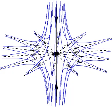
Figure 2.2: Structure of the magnetic field near a potential three-dimensional null-point. The solid black lines marks the spine and the dashed black lines the fan surface.

ideal flux tube no longer be associated with the reconnection process. However, plasma elements associated with thewin-flow and those of thewout-flow will not generally become again magnetically connected (i.e.

‘rejoin’).

We will make extensive use of flux velocities in Chapters 3 and 4 to describe the nature of the 3D reconnection processes under consideration. A further discussion on the existence and uniqueness ofw, together with descriptions of the behaviour of magnetic flux in purely diffusive non-ideal situations, can be found in Wilmot-Smith et al. (2005b).

2.2 Location of Reconnection

Compared with the two-dimensional case, a much wider class of reconnection scenarios may be found in three-dimensional geometries. As already discussed, in 2D, X-points (hyperbolic null points) and O-points (elliptic null O-points) are the only generic null O-points of the magnetic field and it is only possible for reconnection to occur at an X-point, where the flux transport velocity,w, is of a stagnation type close to the null point and has a hyperbolic singularity at that location. Additionally, generation and loss of magnetic flux can both occur at O-points depending on the nature (the direction) of the flux transport velocity near such a point. Moving into in three-dimensions, reconnection may be associated with the presence of a null-point but may also occur when no null-null-points are present; the non-existence of a unique and non-singular flux transport velocity (as discussed in the previous section) and accordant change in magnetic connection no longer relies on the presence of a zero of the magnetic field.

(27)

2.2 Location of Reconnection 18

null-point is an isolated pair of field lines which either diverge or converge from opposite directions onto the null.The fan plane consists of a family of field lines that branch out-of or into the null. The field lines in the fan plane form a separatrix surface that divides regions of differing flux connectivity. If two separatrix surfaces intersect, then their line of intersection will divide four regions of differing flux connectivity. The line is known as a separator.

At isolated null-points two types of reconnection have been identified according to whether the current is aligned with the spine of the null (Pontin et al., 2004) or the fan of the null (Pontin et al., 2005b). The models described in Pontin et al. (2004) and (Pontin et al., 2005b) are kinematic ones in which the equation of motion is neglected, the magnetic field prescribed and the plasma velocity deduced from Ohm’s law (so the term kinematic is used here in a slightly different sense to the traditional use in dynamo theory). In the analysis of reconnection with the current aligned with the spine of the null (Pontin et al., 2004) a simple spiral null point was assumed together with a resistivity localised about the null. The resultant reconnecting plasma flow is found to be non-zero only within the envelope of field lines linking the non-ideal region, rotational in its nature and crossing neither the spine of the null nor the fan plane. In the analysis of Pontin et al. (2005b) a 3D null was taken with a current parallel to the fan plane (and so the spine of the null is not perpendicular to the fan plane) and, again, a localised profile for the resistivity. The reconnecting plasma flow deduced is found to transport magnetic flux across both the spine and the fan of the null, so, in the latter case, transferring flux between domains.

If multiple null points are present in a domain then magnetic separators will be present. Separators form a 3D analogue of the 2D X-point (Lau and Finn, 1990) since they lie at the intersection of four flux domains and, in addition, the field in a perpendicular cross-section has an X-type structure. It is thought that currents will tend to accumulate along separators (Sweet, 1969, Longcope and Cowley, 1996), enabling reconnection to take place there (Lau and Finn, 1990, Priest and Titov, 1996). Several numerical experiments have explored separator reconnection (Galsgaard and Nordlund, 1997, Parnell and Galsgaard, 2004, Haynes et al., 2007) in some detail and observational evidence has been presented by Longcope et al. (2005).

Magnetic reconnection in three-dimensions can also occur in the absence of a null-point. The consider-ations of Section 2.1 show that reconnection may take place whenever any non-ideal terms, such as current concentrations, that can lead to a change in the connectivity of plasma elements are present. An example of reconnection in the absence of a null-point, non-null reconnection, was given by Hornig and Priest (2003). Since much of the work in this thesis also discusses non-null reconnection the findings of Hornig and Priest (2003) are summarised in the Section 2.4.

(28)

2.3 Magnetic Reconnection Rates 19

Figure 2.3: Illustrative example of a situation in which a global change in topology can occur in a 3D domain with no magnetic null points. Two magnetic flux loops exist before reconnection (some particular field lines being illustrated in the left-hand image) but only one flux loop after reconnection (right-hand image). Looking only at a subsection of the process (within the red-box) the change in topology is not evident.

magnetic flux passes through the boundary, and not just an isolated part of the configuration. Such isolated regions are, however, exactly the systems typically analysed in both two and three-dimensional models of magnetic reconnection. Fitting these local models into the global process involves extrapolating the field outside of the model domain (which might be, for example, a cuboid numerical box). However, regardless of the extrapolation used, there will, during the reconnection process, be some change in the topology of the global system. Figure 2.3 provides an illustrative example of the importance of the global system in reconnection.

2.3 Magnetic Reconnection Rates

As previously discussed, reconnection in two-dimensions takes place at an X-type null-point and transfers magnetic flux between topologically distinct domains. The reconnection rate in 2D is a measure of the rate at which flux is transferred between the distinct domains and this rate in turn is given by the value of the electric field at the null point. Traditionally, the rate is expressed in terms of the dimensionless quantity the Alfv´en Mach number through the use of a normalisation of the null point electric field to some characteristic field.

Given the previously mentioned differences between 2D and 3D reconnection the question arises as to how the reconnection rate should be defined, measured and interpreted in 3D? These are still partly open questions. We begin by discussing the case of non-vanishing magnetic field and an isolated non-ideal region (D) in an otherwise ideal environment (Hesse and Schindler, 1988).

For this, consider, as illustrated in Figure 2.4, an isolated non-ideal region D (shaded) with non-vanishing magnetic field and a loop integral where the loop path is along a magnetic field line (shown in red) passing throughDand a material line (blue) in the ideal environment. Integrating the electric field,

E, along this loop and using Faraday’s law (1.6) together with Stokes’ theorem gives

I

C

E_·dl=

Z

S∇ ×

E_·dA=−_dtd

Z

S

B_·dA. (2.10)

(29)

2.3 Magnetic Reconnection Rates 20

Figure 2.4: Example path taken for the loop integral given by equation (2.10) to demonstrate the relation-ship between a non-zero integrated parallel electric field across a localised non-ideal region and magnetic reconnection. The path is taken along a magnetic field line (shown in red) passing though the non-ideal region (shaded) and a comoving line (shown in blue) in the ideal region.

and the only contribution to the loop integral comes from that along the field line passing throughD. We therefore deduce that

d dt

Z

S

B_·dA=−

Z

Ekdl,

where the lineldenotes the field line taken throughD, and so if the integrated parallel electric field along this magnetic field line is non-zero then there must be a change in the magnetic flux enclosed by the loop. The rate of reconnection is then given by the maximum value of this integral across D (and is given a positive value since direction of the normal component to the surface is arbitrary):

dΦrec

dt =

Z

Ekdl

. (2.11)

Thus while the expression for the 2D reconnection rate was given by the electric field at a point in 3D we have the integrated electric field along a line. The formulation (2.11) is consistent with the 2D one with the reconnecting flux in 2D being the 3D flux per unit length in the invariant direction.

Similarly, in a system with reconnection taking place at a magnetic separator, the rate of reconnection is given by the difference in electric potential between the ends of the separator (Longcope and Cowley, 1996). When multiple separators are present in a domain the difference in potential across each must be taken into account. Such a system must be carefully analysed to determine the total reconnected flux since it may allow for flux to be transferred simultaneously into and out of a flux domain at different boundaries (Parnell et al., 2007).

(30)

2.4 An Isolated Non-Null Reconnection Process 21

2.4 An Isolated Non-Null Reconnection Process

In Chapters 3 and 4 we consider non-null reconnection. Much of this work builds on the investigations of Hornig and Priest (2003) and so we now discuss their main findings.

In most of the previous models of reconnection, the non-ideal region is bounded only in two-dimensions and extends to infinity in the third dimension. However, in a realistic model for astrophysical plasma processes, the non-ideal region should be localised in all three dimensions since this is the generic situation in astrophysical plasmas which have length scales along the magnetic field that tend to be much larger than the mean free path.

Hornig and Priest (2003) analysed such a situation in a region of non-zero magnetic field, placing particular emphasis on the evolution of magnetic flux. The model is a kinematic one with kinematic, in this context, referring to the (non-traditional) situation where a magnetic field of a certain form is imposed and a plasma velocity deduced using Ohm’s law. Since the equation of motion is neglected the question as to whether the field can be sustained by the plasma flow is ignored.

The prescribed magnetic field in the model is a linear X-type configuration in thexy-plane with a uniform field component in the third (z) direction and so results in a uniform current. Thus, in order to obtain a localised non-ideal region, a 3D localisation of the resistivity is imposed. In a realistic situation it is expected that finite regions of intense current concentration will be the main cause of such a localisation and that it may be reinforced when the resistivity is enhanced by current-driven microinstabilities. In the model however, the localisation is achieved in this way in order to make analytical progress.

The authors noted that in a general three-dimensional situation, for a specified magnetic field, Ohm’s law may be decomposed into a particular non-ideal solution and an ideal solution:

Enon−id+vnon−id×B = ηj,

Eid+vid×B = 0.

The non-ideal, or particular solution must be deduced from the imposed magnetic field. The localisation ofηjresults in the flows associated with the particular solution being rotational in nature. Identifying the flux tube consisting of all the field lines linking the non-ideal region as a HFT, the non-ideal plasma flows are confined to within the HFT and are rotating in opposite senses above and below the non-ideal region itself, as illustrated in Figure 2.5. Thus the particular solution affects only the flux within the HFT and all the field lines contained within it are continually changing their connections.

(31)

2.5 Aims 22

diffusion

region

_{counter−rotational}

[image:31.595.188.429.120.369.2]

flows

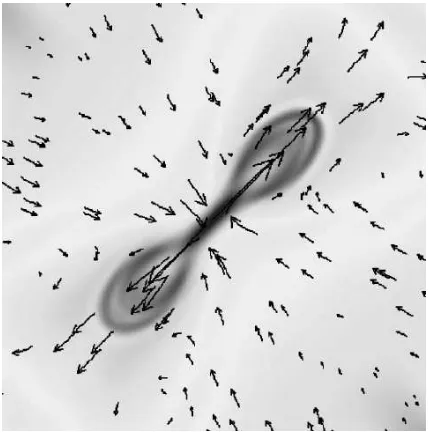
Figure 2.5: Cartoon illustrating the counter-rotational flows (thick solid lines) in the pure solution of Hornig and Priest (2003). The hyperbolic flux tube (HFT) which encloses the localized non-ideal region (shaded) is bounded by the thin solid lines.

their relative strengths, but in either case some flux will be carried by the stagnation flow into the HFT, where reconnection will take place, and then transported away from the region. The combination of the two flows, known as composite solutions may therefore show more similarities to the case of classical 2D reconnection than the particular solutions alone. Thus although the rate of reconnection in both the particu-lar and composite cases is the same (with the ideal solution having no associated parallel electric field), the effect of the reconnection in terms of magnetic flux evolution is quite different.

2.5 Aims

The analysis of Hornig and Priest (2003) left open some important questions. One key feature of the analysis is the ability to impose an arbitrary ideal solution on the non-ideal particular solution. Since this freedom is not present in the 2D kinematic case it may be an inherent feature of a 3D process. However, it may also be the case that in a fully ‘dynamic’ analysis in which the momentum equation is also considered, the freedom disappears since the flowsvnon−idandvidmust also jointly satisfy that equation (Eq. 1.2). In

(32)

2.5 Aims 23

This thesis aims to examine further the nature of 3D non-null reconnection and to address these ques-tions, at least in part. We begin in Chapter 3 by attempting to address the first question, of freedom within 3D reconnection solutions, by building a fully dynamic 3D model. Several of the assumptions taken are the same as those of Hornig and Priest (2003); a stationary solution in a non-null field geometry with a non-ideal region localised in all 3D. We then carry out a perturbation expansion that allows for a splitting of the variables to be made in such a way that comparisons may be drawn with the particular and compos-ite solutions of Hornig and Priest (2003). This enables some circumstances under which the freedom of imposing ideal flows on reconnection solutions exists.

In Chapter 4, we analyse reconnection in a flux-tube where the current-concentration is localised in all three-dimensions, reverting to a kinematic analysis in order to do so. The model uses an elliptic rather than hyperbolic field geometry; whilst the imposed magnetic field of Hornig and Priest (2003) had an X-type structure in thexy-plane and a uniform third component, our model has an O-type structure in thexy-plane (and, again, a uniform third component). The reconnection scenario described corresponds to a situation in which the footpoints of the flux-tubes are spun in opposite directions and the counter-spinning motion results in a localised reconnection region in the centre middle portion of the tube. In the chapter we first carry out an order-of-magnitude analysis that allows an intuitive understanding of the process to be built up before confirming these estimates with a quantitative model.

(33)

Chapter 3

Dynamic Non-Null Reconnection

As discussed in previous section, the analysis of Hornig and Priest (2003) shows several new features of 3D reconnection but it is a kinematic one – the effects of the equation of motion are neglected. The aim of this chapter is to build upon their work by investigating an isolated reconnection process and including the equation of motion in the analysis, so that the model is a fully ‘dynamic’ one. We wish to determine whether the additional freedom to impose an ideal flow on the particular solution arises through the neglect of the momentum equation, or whether it is an inherently 3D effect. The MHD numerical experiments of Pontin et al. (2005a) suggest the latter. In that paper 3D simulations of a non-null reconnection process with a localised non-ideal region are described. Several of the features of the kinematic analysis are observed, in particular a rotational background component to the plasma flow that is of opposite sense on either side of the non-ideal region. Field-lines linking the non-ideal region are found to be continuously changing their connnections.

We take the set of resistive MHD equations (neglecting the energy equation), assume stationarity and imcompressibility, and carry out a perturbation expansion of the equations that allows models of a 3D reconnection process in the absence of a null-point to be built. The assumptions taken in making the expansion are such as to allow Ohm’s law at the zeroth and first orders of the expansion to be written as ideal and non-ideal equations respectively. These equations are coupled together through the momentum equation and so the extent to which this coupling restricts the independence of the zeroth and first order flows (the analogue of the ideal and non-ideal flows in the model of Hornig and Priest, 2003) can be considered.

We begin in Section 3.1 by introducing the expansion technique; the MHD equations are written in dimensionless form, a suitable expansion parameter identified (the Alfv´en Mach number of the flow) and the equations obtained by writing variables in a small-parameter series expansion stated. In Section 3.2 the zeroth order perturbation quantities are chosen in such a way that the full model corresponds to the particular solutions of Hornig and Priest (2003), while in Section 3.3 the zeroth order flow is chosen so that a direct comparison with the composite solutions of Hornig and Priest (2003) is found. The choice of zeroth order flow needed if such a comparison is to be made is found to be somewhat limited and so,

(34)

3.1 Model Setup 25

in Section 3.4, we proceed to examine a more general solution. Although the flow associated with this solution can be viewed as more realistic its form makes significant analytical progress difficult.

The results of this chapter can be found in Wilmot-Smith et al. (2006a) and Wilmot-Smith et al. (2007a).

3.1 Model Setup

We take the stationary incompressible resistive MHD equations and non-dimensionalise by setting

B=BeB′,v=vev′,E=veBeE′,j=

Be

µLe

j′, p=B

2

e

µ p ′_,_r₌_L

er′,

where all the dashed quantities are of order one, andBe, Le, andveare the typical magnetic field strength,

length-scale and plasma velocity. Thus Ohm’s law becomes

E′+v′_×B′ =vAe ve

ˆ

ηj′, (3.1)

wherevAeis the typical Alfv´en speed of the plasma, and

ˆ

η= η

µLevAe ,

is the inverse Lundquist number.

The equation of motion is

Me2(v′· ∇′)v′ =−∇′p′+j′×B′, (3.2)

whereMe=ve/vAeis the Alfv´en Mach number. For simplicity we choose to neglect here the effects that viscosity and other forces (such as gravity) might have on the solutions. The remaining MHD equations are given by

∇′_×_B′₌_j′_, _(3.3)

∇′×E′=0,

∇′·B′ = 0,

∇′·v′= 0.

Having non-dimensionalised in this way we must now choose a suitable small parameter in which to carry out the expansion. For this we choose the Alfv´en Mach numberMeof the flow, and therefore must

takeMe ≪ 1. Low Mach number expansions have already been employed in the development of 2D

reconnection theories – for example in the linear reconnection models of Priest and Forbes (1986) and their extention by Jardine and Priest (1988). In this case the expansion of variables is assumed as follows:

(35)

v′=v1+Mev2+Me2v3+· · ·,

j′=Mej1+Me2j2+Me3j3+· · · ,

E′ = E0+MeE1+Me2E2+· · ·

= −∇′φ0−Me∇′φ1−Me2∇′φ2+· · ·,

p′ =p0+Mep1+Me2p2+· · ·.

where all the quantitiesBi,vi,ji,Ei, φi, pi are dimensionless. Note that we have labelled the first term

in the expansion ofv′ with the index1 and have also takenj0 = 0, so that the lowest order magnetic field is potential, an assumption that is crucial in allowing us to find analytical solutions to the equations. Substituting these expansions into both Ohm’s law and the equation of motion and comparing powers of Mewe find that at zeroth order the equation of motion is satisfied withp0a constant, while Ohm’s law is

given by

E0+v1×B0= ˆηj1. (3.4)

At first order we obtain

E1+v1×B1+v2×B0= ˆηj2, (3.5)

0=−∇′p1+j1×B0. (3.6)

At second order the equations become

E2+v1×B2+v2×B1+v3×B0= ˆηj3, (3.7)

(v1· ∇′)v1=−∇′p2+j2×B0+j1×B1, (3.8)

while at third order we have

E3+v1×B3+v2×B2+v3×B1+v4×B0= ˆηj4, (3.9)

(v2· ∇′)v1+ (v1· ∇′)v2=−∇′p3+j3×B0+j2×B1+j1×B2. (3.10)

It is clear that a natural coupling exists not between the same ordered equations for Ohm’s law and the equation of motion, but rather between Ohm’s law at a given order, and the equation of motion at the next order. Thus to solve the system we will have to consider, for example, equations (3.4) and (3.6) together, and (3.5) and (3.8) together.

We set

B0=b0(ky, kx,1), (3.11)

whereb0and k are constants andk >0. Thus our basic state is an X-type current-free equilibrium in the xy-plane, superimposed on a uniform field in thez-direction. The field structure is illustrated in Figure 3.1. The field is assumed to be reconnecting slowly (v≪vA), and is similar to that taken by Hornig and Priest

(36)

–0.4

0 0.2 0.4

x –0.4

–0.2 0 0.2 0.4

y –2

–1 0 1 2

z

Figure 3.1: Illustration of some particular field lines indicating the structure of the magnetic fieldB0.

With this choice of field configuration we can analytically integrate the equations

∂X(s)

∂s =B(X(s))

to find the equationsX(x0, s)of the field line passing through the initial pointx0. The components of

X(x0, s)are given by

X=x0cosh(b0ks) +y0sinh(b0ks),

Y =y0cosh(b0ks) +x0sinh(b0ks), (3.12)

Z=b0s+z0.

with the inverse mappingX0(x, s), being given by

X0=xcosh(b0ks)−ysinh(b0ks),

Y0=ycosh(b0ks)−xsinh(b0ks), (3.13)

Z0=−b0s+z.

The parametersparameterizes the magnetic field line and is related to the distance,λ, along field lines by ds=dλ/|B|.

(37)

3.2 Particular Solutions 28

3.2 Particular Solutions

In this section we consider the implications of the first-order solution alone, by assumingv1 =0. Ohm’s law at zeroth order becomesE0=0, while the equation of motion is safisfied at zeroth and first order with p0andp1 constants. This assumption results in the solutions obtained being equivalent to the particular solutions of Hornig and Priest (2003) (with the first order Ohm’s law the non-ideal equation), but now also satisfying the momentum equation. For these particular solutions it is first necessary to consider equations (3.5) and (3.8) together:

E1+v2×B0= ˆηj2, (3.14)

0=−∇′p2+j2×B0. (3.15)

Under these assumptions it is at fourth order that the inertial term first appears, and thus the dynamic effects in our particular solution are primarily the Lorentz force and the pressure gradients. Here we will consider the implications of two different forms for the non-ideal terms,ηˆj2, with special emphasis placed on the resulting plasma flows and rate of reconnected flux.

Localisation of the non-ideal termηˆj2can be achieved through a localisation in three dimensions of eitherη, or ofˆ j2, or, in the physically most realistic situation, through a localisation of both terms. The important quantity in determining the main results presented here isφ1, which is dependent only on the localisation of the productηj2kˆ , and not on how the localisation is realised. As a simplification and in order to allow for analytical solutions we here choose to prescribe a localisation of the resistivityη. Thisˆ

assumption was also taken by Hornig and Priest (2003) where a hyperbolic field similar to that given by (3.11) resulted in a uniform current in thezˆ-direction. By taking the curl of (3.15) we obtain

(B0· ∇)j2−(j2· ∇)B0=0,

which, assumingj2=j2(x, y)zˆ, gives(B0· ∇)j2=0, i.e.j2as constant along field lines ofB0:

j2=f(x2−y2)zˆ. (3.16)

There are a number of ways to choosef(x2₋_y2₎_{, two of which we examine here. In Section 3.2.1 we} takef to be uniform, as was the case in Hornig and Priest (2003). In Section 3.2.2 we instead assume a form such that the currentj2is localised along separatrices ofB0, which is motivated by the numerical experiments of Pontin et al. (2005a) where a such a current was observed.