DOI 10.1007/s10827-017-0655-7
A mean field model for movement induced changes
in the beta rhythm
´
Aine Byrne1 ·Matthew J Brookes2·Stephen Coombes1
Received: 21 October 2016 / Revised: 27 March 2017 / Accepted: 31 May 2017 © The Author(s) 2017. This article is an open access publication
Abstract In electrophysiological recordings of the brain, the transition from high amplitude to low amplitude sig-nals are most likely caused by a change in the synchrony of underlying neuronal population firing patterns. Classic examples of such modulations are the strong stimulus-related oscillatory phenomena known as the movement related beta decrease (MRBD) and post-movement beta rebound (PMBR). A sharp decrease in neural oscillatory power is observed during movement (MRBD) followed by an increase above baseline on movement cessation (PMBR). MRBD and PMBR represent important neuroscientific phe-nomena which have been shown to have clinical relevance. Here, we present a parsimonious model for the dynamics of synchrony within a synaptically coupled spiking network that is able to replicate a human MEG power spectrogram showing the evolution from MRBD to PMBR. Importantly, the high-dimensional spiking model has an exact mean field description in terms of four ordinary differential equations that allows considerable insight to be obtained into the cause of the experimentally observed time-lag from move-ment termination to the onset of PMBR (∼0.5 s), as well
Action Editor: Maxim Bazhenov
Aine Byrne´
1 Centre for Mathematical Medicine and Biology,
School of Mathematical Sciences, University of Nottingham, University Park, Nottingham, NG7 2RD, UK
2 Sir Peter Mansfield Imaging Centre, School of Physics
and Astronomy, University of Nottingham, University Park, Nottingham, NG7 2RD, UK
as the subsequent long duration of PMBR (∼ 1−10 s). Our model represents the first to predict these commonly observed and robust phenomena and represents a key step in their understanding, in health and disease.
Keywords Post-movement beta rebound·Movement related beta decrease·Neural mass·Synchrony·Power spectra·Magnetoencephalography·MEG·
Electroencephalography·EEG·Mean field
1 Introduction
conductance based modelling, large scale network simula-tions and theories for understanding coupled oscillators, as recently surveyed in Ashwin et al. (2016). For questions that relate to understanding the coarse grained activity of either synaptic currents, mean membrane potentials or population firing rates, it is more natural to appeal to neural mass mod-els, as reviewed in Coombes (2010). Indeed the latter have proven especially fruitful in providing large scale descrip-tions of how neural activity evolves over both space as well as time (Coombes et al.2014; Pinotsis et al. 2014). How-ever, these two approaches are dangerously close to creating a dichotomy so that there is no ideal computational mod-elling framework for understanding the role of spike-timing in generating localised brain rhythms.
A case in point that challenges the modelling tools cur-rently available to us is the work of Jasper and Penfield (1949) who showed that beta rhythms generated from the motor cortex are suppressed during voluntary movement. This phenomenon is known as movement related beta decrease (MRBD). It wasn’t until some years later that the post-movement beta rebound (PMBR) (a temporary rise in amplitude of beta oscillations following movement cessa-tion) was discovered (Riehle and Vaadia2004; Pfurtscheller et al. 1996; Jurkiewicz et al. 2006). MRBD usually lasts for approximately 0.5 seconds and PMBR can last for up to several seconds. MRBD and PMBR are extremely robust, with clear amplitude changes in individual subjects and trials (Pfurtscheller and Lopes da Silva 1999). Inter-estingly, similar effects have been seen in studies where the subject is asked to think about moving, without carry-ing out the movement (Schnitzler et al.1997; Pfurtscheller et al. 2005). These beta band modulations are believed to be caused by changes of synchrony within a relatively localised region of motor cortex (Stanc´ak and Pfurtscheller 1995). Hence, MRBD is regarded as a special case of event-related desynchronisation (ERD) and PMBR a special case of event-related synchronisation (ERS).
Multiple papers have employed a large number of care-fully controlled paradigms, in humans and animals to further investigate beta rebound phenomena and their mod-ulations by tasks (see Cheyne2013; Kilavik et al.2013for reviews). However, despite the robust nature of the beta task induced decrease and post stimulus rebound, the effect itself is relatively poorly understood and, at the time of writing, there has been, to our knowledge, no computational model capable of describing the beta rebound. In general, high amplitude beta oscillations are thought to reflect inhibition (Cassim et al.2001; Gaetz et al. 2011), a hypothesis sup-ported by quantifiable relationships between beta amplitude and local concentrations of the inhibitory neurotransmit-ter gamma aminobutyric acid (GABA) (Gaetz et al.2011; Hall et al. 2011; Jensen et al. 2005; Muthukumaraswamy et al. 2013). This means that the observed MRBD might
reflect an increase in processing during movement planning and execution and the PMBR might reflect active inhibition of neuronal networks post movement (Alegre et al. 2008; Solis-Escalante et al.2012). An alternative, but not mutually exclusive hypothesis which has been proposed by Donner and Siegel (2011) (also outlined in Liddle et al.2016) is that the beta signal, in part, represents long range integration across multiple brain regions (see also Liddle et al.2013). Indeed this is a hypothesis supported by some evidence sug-gesting that large scale distributed network connectivity is mediated by beta oscillations (Brookes et al. 2011; Hall et al.2014; Hipp et al.2012).
To describe beta rebound we are faced with modelling a mesoscopic brain scale and in particular the changes of synchrony within a population of say 106−7excitatory pyra-midal cells and their associated inhibitory interneurons. A neural mass model would be ideal for this scale, if the question of interest related to rate rather than spike, which suggests instead a simulation of a spiking neural network model. Unfortunately the latter can be notoriously hard to gain insight from for very large numbers of neurons. Ideally we would have access to a statistical neurodynamics provid-ing a bridge between the two levels of description. This is an open mathematical problem. However, recent progress in obtaining a mean field reduction for a very specific choice of large scale spiking model has been made, and is ideally suited as a basis for breaking the dichotomy noted above. The single neuron model of choice being either aθ-neuron (So et al. 2014; Luke et al. 2013) or a (formally equiva-lent) quadratic integrate-and-fire (QIF) neuron (Paz´o and Montbri´o1009), and the coupling being global and medi-ated by pulses (namely instantaneous synapses). Given the dense connections of connections in cortex on small scales (Klinshov et al.2014) the global coupling assumption is not so restrictive for our purposes, though the assumption of fast synapses should be relaxed to incorporate more real-istic post synaptic responses. This is precisely the issue we address here to develop a model capable of explaining MRBD and PMBR.
the Kuramoto measure of synchrony (for the phase descrip-tion). Importantly we show in Section4that the response of the mean field model to stimulation leads to spectro-grams with all of the key features observed in MRBD and PMBR. Finally in Section5we emphasise the benefits of this new type of neural mass model, capable of tracking not only changes in firing rate but also coherence within a pop-ulation, in describing cortical rebound, as well as discuss natural extensions to our initial single population approach.
2 MRBD and PMBR: a recapitulation
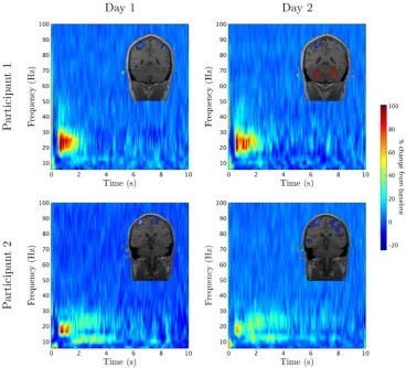
Beta band modulation is robust across subjects; occurring during internally and externally cued movements, as well as during somatosensory stimulation. To demonstrate this, for somatosensory stimulation, we carried out a series of median nerve stimulation experiments on two healthy par-ticipants. The participant’s median nerve was stimulated at the wrist using a constant current stimulator and the neu-rological response was measured using MEG (for more details on the experimental design see AppendixA). The experiment was repeated on separate days to determine how reproducible the results were. Figure1shows the relative
time-frequency spectrograms for two such experiments for each participant, where baseline activity has been sub-tracted. The top line represents the data for participant 1 and the bottom line represents participant 2. For each case there is a 10–20% decrease in power for∼ 0.5 s, demonstrating MRBD. At∼ 0.5 s there is a 60–100% increase in power, exemplifying PMBR. Although the comparison between participants shows dissimilarities in the shape and length of PMBR, the strength and timing of both the MRBD and PMBR are comparable. Importantly, the similarity between each participant’s time-frequency spectrogram on separate days is compelling.
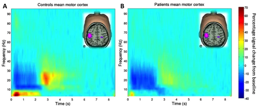
Recent work, reviewed in Brookes et al. (2011, 2012) and Robson et al. (2015), has begun to show the poten-tial importance of beta band modulation. For example, Fig.2(recreated with permission from Robson et al.2015) shows relative time-frequency spectra depicting the changes in neural oscillations in sensorimotor cortex in response to a cued finger movement task. The left hand panel (a) shows the case for healthy individuals. The time-frequency spectrum is extracted from a location of interest in left pri-mary motor cortex. Notice that in the beta band, the MRBD and PMBR are observed clearly. The right hand panel (b) shows the case for patients with schizophrenia. Note the
Fig. 1 Robust beta rebound for median nerve stimulation: Time-frequency spectrograms showing the percentage change from baseline of the activity in the motor cortex, for 2 participants on two separate days. Thetop rowshows the results for participant 1 and thebottom row
[image:3.595.176.545.381.715.2]A
B
Fig. 2 The beta rebound and its disruption in patients with schizophre-nia: (a) Time-frequency spectrograms showing changes in the ampli-tude of neural oscillations, in contralateral sensorimotor cortex, when subjects execute a 2s finger movement. Note that, in the beta band the loss in oscillatory power during movement is accompanied by
an increase in power on movement cessation. (b) Equivalent time-frequency spectrogram in patients with schizophrenia. Note the sig-nificant reduction in PMBR (Figure reproduced with permission from Robson et al.2015.)
significant reduction in PMBR. Furthermore, this same study showed that the magnitude of the beta rebound corre-lated significantly with the severity of ongoing symptoms of schizophrenia, thus highlighting direct clinical relevance to the measurement. This is just one example of how beta band oscillations have been identified as a potential biomarker of disease; other examples include Parkinson’s Disease (Timmermann and Florin2012). In addition, the robustness of MRBD and PMBR has meant that they have also been
used in neuroscience applications ranging from brain com-puter interfaces (Pfurtscheller and Solis-Escalante2009) to markers of neural plasticity (Gaetz et al.2010; Mary et al. 2015). It is also noteworthy that the beta band power loss and rebound, whilst commonly thought of as being observ-able in the sensorimotor cortex, is not a sole property of the sensorimotor system. For example, Fig.3shows instances of observation of very similar phenomena in other corti-cal areas. Figure 3a shows the time-frequency oscillatory
Fig. 3 Task induced beta band decrease and rebound phenomena in other cortical regions: (a) Time-frequency dynamics in a network of brain areas including bilateral insula. The task involved visual stimuli that were relevant and irrelevant to the task. Note the sig-nificant reduction and rebound in beta oscillations in the relevant condition. (Reproduced with permission from Liddle et al. 2016.)
[image:4.595.82.518.56.234.2] [image:4.595.309.542.451.645.2]dynamics of a network of brain areas encapsulating bilat-eral insula cortex, throughout a cognitive task (Liddle et al. 2016; Brookes et al.2012). The task itself involves presen-tation of a series of visual stimuli; some stimuli are relevant to the task, others irrelevant. Subjects were asked to respond if the relevant stimuli match some predetermined condition. Note here that only the non-target stimuli are shown (mean-ing that the subjects did not actually make a response). In the relevant condition, clear beta modulation is observed with a decrease in amplitude followed by a rebound above base-line. Furthermore, this effect was also shown to be abnormal in schizophrenia, again demonstrating its clinical relevance. Figure 3b shows the case for simple sensory stimulation of the visual cortex (Stevenson et al.2011). Here, subjects were asked to passively view a drifting visual grating; the figure shows the envelope of beta band oscillations through-out the task. Note again the clear structure with a loss in beta amplitude during stimulation and an increase on stim-ulus cessation. These represent two simple examples which show that the beta band effect is not simply a property of the sensorimotor system, but rather is a ubiquitous effect that is observed robustly across many cortical regions.
The above indicates that stimulus related beta power loss and post stimulus rebound are generally observable effects, seen in many cortical areas, during both sensory and cogni-tive tasks. Further, the reduction of rebound in disease has been robustly demonstrated. Thus, the generation of new mathematical models from which we can accurately predict task induced beta band dynamics are of interest.
3 A mean field model for spiking networks
There are a now a plethora of single neuron models for describing the spiking dynamics of cortical cells, many of which are extensions of the basic Hodgkin-Huxley model to incorporate nonlinear ionic currents that allow low fre-quency firing in response to constant current injection. Importantly mathematical neuroscience has identified a number of mechanisms that can generate ‘f-I’ curves with this property, with perhaps the most well known being the saddle-node on an invariant circle (SNIC) bifurcation (Ermentrout and Kopell1986). This has led to the formu-lation of the elegantθ-neuron model (or Ermentrout-Kopell canonical model) which can mimic the firing and response properties of a cortical cell with a purely one dimensional dynamical system evolving on a circle. In a certain limit this is formally equivalent to the quadratic integrate-and-fire (QIF) model, also designed explicitly for understanding the generation of low firing rates in cortex (Latham et al.2000). Given the simplicity of these models they are a natural can-didate for cortical network studies, not only because they are computationally cheap, but because there is more chance
to develop a statistical neurodynamics for such models than their biophysically complicated conductance based counter-parts. Indeed mean field models for globally pulse-coupled networks have recently been developed by Luke et al. (2013) forθ-neuron models, and by Montbri´o et al. (2015) for QIF models. To make these models more relevant to the interpre-tation of brain imaging signals, and in particular EEG and MEG, it is vital to augment the networks with more real-istic forms of synaptic interaction and to move away from the overly restrictive assumption of fast pulsatile synaptic currents.
We consider a network of N QIF neurons each with a voltage vi, fori = 1, . . . , N, evolving according
accord-ing to the followaccord-ing set of coupled ordinary differential equations (ODEs):
C d
dtvi=ηi+κv 2
i +Ii, i=1, . . . , N. (1)
Here C is a capacitance,ηi is a constant current drive,κ
is a proportionality constant, which from now on (without loss of generality) will be set to unity, andIiis the synaptic
current,
Ii =g(t)(vsyn−vi), (2)
whereg(t) represents a common time-dependent synaptic drive, which we shall take to arise through global coupling. This acts to push the voltage toward the synaptic reversal potentialvsyn. If the synaptic current is positive (negative) we say that the synapse is excitatory (inhibitory). The QIF network has discontinuous trajectories since whenever vi
reaches a threshold value vth it isresetto the valuevreset. This firing condition is also used to define an implicit set of firing times according tovi(Tim)=vth, whereTimdenotes
the mth firing time of the ith neuron. These in turn can be used to generate a set of conductance changes for the
ith neuron that we write in the form m∈Zs(t −Tim), wheres(t)is a fixed temporal filter. For a globally coupled network, with strength of synapse k/N, the total synaptic conductance change at each neuron is then
g(t)= k N
N
j=1
m∈Z
s(t−Tjm). (3)
For fast pulsatile interactions we may sets(t)=δ(t), where
δis a Dirac-delta function. For a more realistic form describ-ing a normalised post synaptic potential (PSP) with an exponential decay we may sets(t)=αe−αt(t), whilst for
a more general PSP with both a rise and fall time we would sets(t)=(1/α1−1/α2)−1[α1e−α1t−α2e−α2t](t). Here (t)is a Heaviside step function included to enforce causal-ity, and the parametersα,α1,2 are decay rates. Exploiting
Table 1 Synaptic filtering: Examples of differential operators and their corresponding temporal filters
Q s(t )
1 δ(t )
1+1
α
d dt
αe−αt(t)
1+ 1
α1
d dt 1+
1
α2
d dt
1
α1−
1
α2
−1
α1e−α1t−α2e−α2t(t)
The first example shows pulsatile coupling, where no synaptic filter-ing has been applied to the incomfilter-ing spike. The second type of filter shown is an exponentially decaying function, which accounts for the slow decay of the instantaneous pulse. It does not however account for the time it take a synapse to process the incoming action poten-tial, increasing instantaneously to the maximum value as soon as the spike arrives. The last example takes into account this synaptic pro-cessing delay, increasing smoothly to its peak value and then decaying exponentially back to zero. Note that(t)represents the Heaviside function
a linear differential operatorQthen we may also writegas the solution to the ODE system
Qg(t)= k N
N
j=1
m∈Z
δ(t−Tjm). (4)
For the corresponding operator Q to the choice of s see Table 1. For the rest of this paper we shall work with the choice s(t) = α2te−αt, describing the so-called
α-function. This can be obtained from the difference of exponentials form described above in the limitα1,2 → α,
so that the corresponding differential operatorQis
Q=
1+ 1
α
d dt
2
. (5)
Thus Eqs. (1)–(5) define our spiking model. This is fur-ther illustrated in Fig. 4 for an all-to-all coupled neural
network, with an inset showing the single neuron dynam-ics. Each neuron generates a train of spikes described by a sequence of Dirac-delta functions that are then filtered with the kernels(t) to generate a synaptic current according to Eq. (2). From this one may in principle use Maxwell’s equa-tions to determine the magnetic field that would underly an MEG-like signal. However, for simplicity we shall take the average network current to be a proxy for this physiological signal. This is given explicitly byg(t)(vsyn−V (t)), where
V (t)= 1 N
N
j=1
vj(t), (6)
which describes the average membrane potential.
For a single uncoupled neuron (k=0) it is a simple mat-ter to show that, whenvth → ∞ andvreset → −∞, the frequency of oscillation is given by 2√ηi/C. For further
simplicity we shall work with these choices for the values of
vthandvreset. From now on we shall chooseηito be random
variables drawn from a Lorentzian distributionL(η)with
L(η)= 1
π(η−η0)2+ 2, (7)
whereη0is the centre of the distribution and the width at half maximum. For simplicity we will consider the aver-age frequency of oscillations ω0 = 2√η0/C as a single parameter, distributed with a width at half maximum ω=
2√ /C. In the coupled network, and if the frequencies of the individual neurons are similar enough, then one may expect some degree of phase locking (ranging from synchrony to asynchrony), itself controlled in part by the time-to-peak, 1/α, of the synaptic filter.
As shown in Fig. 5, for a model with predominantly inhibitory connections, we see patterns of coherent spik-ing. The degree of coherence is mainly controlled by the degree of heterogeneity of the constant current drives ηi.
Fig. 4 Neural network: The diagram on the right shows an all-to-all coupled network. The
zoom on the leftshows each of the components of Eqs. (1), (3) and (4). Thetop plot of the zoom
shows the shape of the synaptic filter for the case thats(t)is an
α-function:s(t)=α2te−αt, where 1/αis thetime-to-peak.
Iiis the total synaptic current
that enters the cell body andvi
is the voltage of the cell which oscillates as shown in themiddle plot. The corresponding output spike train is given by a sequence of Dirac-delta functionsδi=m∈Zδ(t−Tim),
[image:6.595.179.545.522.714.2]Fig. 5 Quadratic integrate-and-fire dynamics: Thetop plotshow a raster plot depicting the spike times for a sample of size 100 in a network of 500 QIF neurons. Thelower plotsshow the mean field vari-ables; the firing raterand the average voltageV. Parameter values are chosen such that the system exhibits partial synchrony;ω0 = 0.269 Hz, ω=0.042 Hz,vsyn= −10 mV,k=0.105, 1/α=35 ms,C= 30 mF
In this figure we also track the evolution of two macro-scopic order parameters. These are respectively the average membrane potential, given by Eq. (6), and the instantaneous mean firing rater:
r(t)= 1 N
N
j=1
m∈Z
δ(t−Tjm). (8)
For large N both the order parameters V and r show a smooth temporal variation. In the case of synchrony we would expect these mean field signals to show a periodic temporal variation, essentially following a trajectory rem-iniscent of a single QIF neuron receiving periodic drive, whilst for an asynchronously firing population these mean field signals would be constant in time (modulo finite size fluctuations). To quantify the degree of coherence (or phase-locking) within an oscillatory population it is convenient to use a Kuramoto order parameter. First though it is necessary to recast the model in terms ofphasevariables.
Given the well known link between the QIF neuron and theθ-neuron it is natural to introduce the phase variableθi∈
[−π, π )according tovi =tan(θi/2)(so that cosθi =(1−
v2i)/(1+vi2)and sinθi = 2vi/(1+v2i)). In this case we
arrive at theθ-neuron network
C d
dtθi=(1−cosθi)+(1+cosθi)(ηi+gvsyn)−gsinθi, (9)
Qg= 2 C
k N
N
j=1
P (θj). (10)
HereP (θ ) = δ(θ −π ) and is periodically extended such that P (θ ) =P (θ +2π ), and we have used the result that
δ(t−Tjm)=δ(θj(t)−π )| ˙θj(Tjm)|. The network defined by
Eqs. (9) and (10) describes a set ofN phase variables inter-acting via spike triggered currents every time thatθj passes
throughπ. We will only consider the case thatθj increases
throughπ(so that spikes are only generated on the upswing of the corresponding voltage variable). In the absence of synaptic coupling an isolated θ-neuron supports a pair of equilibriaθ±, withθ+ <0 andθ− >0 forηi <0, and no
equilibria forηi>0. In the former case the equilibria atθ+
is stable and the one atθ− unstable. In neurophysiological terms, the unstable fixed point atθ− is a threshold for the neuron model. Any initial conditions withθ∈(θ+, θ−)will be attracted to the stable equilibrium, while initial data with
θ > θ−will make a large excursion around the circle before returning to the rest state. For ηi > 0 theθ-neuron
oscil-lates with frequency 2√ηi/C. Whenηi = 0 theθ-neuron
is poised at a saddle-node on an invariant circle (SNIC) bifurcation.
As well as naturally providing a phase variable the θ -neuron network is more straight forward to simulate as the model has continuous trajectories on anN-torus (and there is no need to handle the discontinuous reset conditions). The Kuramoto order parameter is then defined as
Z(t )= 1 N
N
j=1
eiθj(t)≡R(t)ei(t). (11)
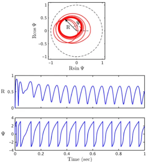
Here R provides a measure of the degree of coherence within the network andis the average phase. If a popula-tion is perfectly synchronised thenR = 1 and similarly if the system is perfectly asyncronous thenR = 0. In Fig.6 we show a sequence of snapshots of the Kuramoto order parameter for the dynamics shown in Fig.5, as well as the time evolution of the degree of coherence.
[image:7.595.53.289.58.385.2]Fig. 6 Theta neuron dynamics: Thetop set of plotsshow the phases of the individual neurons, represented by the coloured dots, at 3 different values of timet. The colour of each neuron has no intrinsic meaning, and is used merely to aid in distinguishing the dots. The phase of each neuron is the angular position of the coloured dot. Theblack dotin the centre represents the Kuramoto order parameterZ=Rei. In thetop left plotthe system is completely asynchronous andZ 0. Thetop
middle plotdemonstrates that the length from the centre of the disk to theblack dotrepresentsR, the population synchrony, and, the aver-age phase, is represented by the angular position of the black dot. The
top right plotshows the system at a later point in time. Thelower plots
showRandas a function of time. One observes that both the popu-lation synchrony and average phase continuously oscillate. Parameter values as in Fig.5
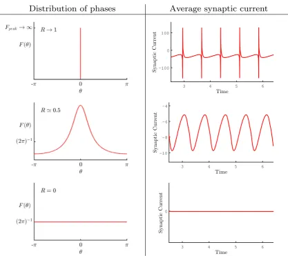
infinite size limit to an explicit finite set of nonlinear ODEs. These describe the macroscopic evolution of the system, in terms of the Kuramoto order parameter for synchronisa-tion, as long as the distribution of phases is at most single peaked. In essence the ansatz is well suited to describing systems which dynamically evolve between an incoherent asynchronous state and a partially synchronised state, which is often the case in systems with interactions that are pre-scribed by harmonic functions, such as found in Eq. (9). To illustrate the type of network evolution that can be gener-ated with different values of synchrony, see Fig.7. Here we show some plots of the phase distribution for different val-ues of the network coherence as well as the average network current that would be produced.
Interestingly, Montbri´o et al. have recently shown how to move between order parameters for the phase and volt-age descriptions with the use of a conformal transformation (Montbri´o et al.2015). If we introduce the complex order parameter for the voltage description as
W=π Cr+iV , (12)
then the following transformation allows one to switch perspectives and obtain the order parameter for the volt-age description in terms of the Kuramoto order parameter as
W = 1−Z
1+Z, (13)
whereZdenotes the complex conjugate ofZ. Importantly the OA ansatz can also be used to obtain a mean field model in the presence of non-pulsatile synaptic, extending the approaches in Luke et al. (2013) and Montbri´o et al. (2015). In AppendixBwe show that this yields the mean field model described by the fourth order ODE system:
C d
dtZ = −i
(Z−1)2
2 +
(Z+1)2
2
− +iη0+ivsyng
−Z2−1
2 g, (14)
[image:8.595.143.452.58.351.2]Fig. 7 Distribution of phases: Figure illustrating the distribution of phasesF (θ )in the largeNlimit and the average synaptic current for different values of the population coherenceR. For simplicity we have fixed the choice of time so that(t )=0. When the population is com-pletely synchronous (R=1) all of the neurons have the same phase and as a result all of the neurons fire together so thatF (θ ) = δ(θ )
and the average synaptic current is veryspiky. In the regime where
R0.5 the phases are more distributed. Although a dominant phase can be clearly identified (by the peak value) not all neurons have this
phase. The OA ansatz gives the shape of the distribution in the form
F (θ )=(2π )−1(1−|Z|2)/(|eiθ−Z|2). This spread in the phase
distri-bution acts to smooth out the spikes in the average synaptic current to create a smooth oscillatory signal. When the population of neurons is completely asynchronous there is no dominant phase and every phase is equally probable so thatF (θ )=1/(2π ). In this case all of the neu-rons fire at different times with their phases uniformly distributed to yield a constant synaptic current. Note that the peak in the distribution of phases move as the system evolves with time with a velocity˙
HereH (Z)is a global state dependent drive to the popula-tion given by
H (Z)= 1 Cπ
1− |Z|2
1+Z+Z+ |Z|2, |Z|<1. (16)
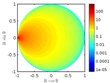
A plot of this scalar function of a complex variable is shown in Fig.8. It is illuminating to expressH as function ofW
using (13) from which we find
H (W )= 1 Cπ
W+W
2 =r. (17)
Hence we may interpretH (Z)as the firing rate of the popu-lation that drives the global synaptic current. Figure8shows
Has a function ofZ. As expectedHtakes its highest value whenZ eiπ, corresponding to high synchrony where all of the neurons fire and reset at the same time.
Figure9shows results for a simulation of 500 theta neu-rons (red) and a simulation of the reduced mean field model (blue). It is strikingly clear that the two simulations agree very well. If the size of the population in the large scale simulations is reduced then one can begin to see finite size fluctuations, as expected. The macroscopic order parame-ters(r, V )in the reduced mean field model are plotted in Fig.10. Unsurprisingly they behave similarly to the corre-sponding order parameters for the large scale simulations plotted in Fig.5. Likewise, the mean field representation of
[image:9.595.86.504.54.425.2]Fig. 8 Plot ofH: Density plot showingHas a function of the complex numberZ=Rei. AsHcorresponds to the firing rate it takes a high
value nearZ=eiπ, this corresponds to highly synchronous behaviour
where all of the phases of the neurons go throughπsimultaneously
shown in Fig.6. For a further discussion of the bifurcation structure of this model see Coombes and Byrne (2017).
4 A mechanistic interpretation of movement induced changes in the beta rhythm
In Section2we demonstrated how an externally cued thumb movement caused a∼0.5 s decrease in beta band power fol-lowed by a∼2−4 s increase in beta band power, typifying MRBD and PMBR, respectively. The median nerve stim-ulation lasts∼ 50 ms, however the evoked response lasts significantly longer. Upon examining the time-frequency spectrograms in Fig.1we observed an increase in low fre-quency activity att =0, which appears to last for∼0.3− 0.4 s, corresponding to the transduced median nerve stimu-lation and corresponding movement. We base the design of the external drive on this transduced signal.
[image:10.595.74.263.56.198.2]We model the transduced signal as a temporally filtered drive A = A(t) that is received by every neuron in the
Fig. 10 Mean field reduction for a QIF network: Time series for the mean field variableW=π Cr+iV, whereris the population firing rate andVis the average voltage. Comparing these plots to the corre-sponding plots for a 500 neuron simulation in Fig.5it is clear to see that they agree well. The finite size fluctuation forV are quite appar-ent when comparing the results for the large scale simulation to those of the reduced mean field model. However, the overall behaviour is similar. Parameters as in Fig.5
model. In this case the dynamics ofZobey (14) under the replacementη0 → η0+A, withQDA(t) = (t), where
QD is the differential operator obtained fromQ in Eq.5
under the replacementα → αD, and(t)is a rectangular
pulse, (t) = (t)(τ −t), where can be inter-preted as the strength of the drive. Note that the pulse is not applied until after transients have dropped off. As the evoked response in the experimental data last for∼0.3−0.4 s we setτ =0.4 s.
Fig. 9 Validity of reduction: Comparison between the reduced mean field network (blue) and simulation a network of 500θ-neurons (red). Phase plane for the Kuramoto order parameterZ=Reiis shown
on theleftand the phase plane for the synaptic conductanceg
and its derivativeg is shown on theright. Parameter values as in Fig.5
-1 -0.5 0 0.5 1
-1 -0.5 0 0.5
[image:10.595.304.545.58.293.2] [image:10.595.175.543.532.713.2]Fig. 11 Mean field reduction for aθ-neuron network: Phase plane of the Kuramoto order parameterZ, showingR(t)and(t ), as well as a time series for bothRand. Once again the plots match very well with the corresponding plots for the simulation of 500θ-neurons in Fig. 6. Interestingly even the initial behaviour is well matched. Parameter values as in Fig.5
Figure12shows the phase plane for the Kuramoto order parameterZ=Rei, as well as a time series for the within
population synchronyR, in response to the drive described above. The colours correspond to the different time periods; before drive (blue), during drive (red), after drive (green). The system oscillates in partial synchrony withR oscillat-ing between∼ 0.05−0.6 in the absence of drive. Once the drive is switched on the amplitude of these oscillations decreases and hence the power is also reduced, correspond-ing to MRBD. Note that the frequency also increases durcorrespond-ing this period. After the drive is switched off the level of coher-ence is increased as Z is drawn towards the edge of the unit disk before spiralling back to the original limit cycle, corresponding to PMBR. Importantly the system does not rebound untilt 0.5 s as seen in the real data. It should be noted that the stimulus corresponds to∼80% of this time to rebound, however as the evoked response is present in ∼60−80% of the∼0.5 s of MRBD in the real data we believe that this is a good fit.
The corresponding response of the synaptic current is shown in Fig.13. The time series (left) shows that when the drive is switched on the synaptic current is reduced, how-ever the neurons are now also receiving a strong excitatory current in the form of the drive. There is a large increase in the amplitude of the oscillations of the synaptic current at
Fig. 12 Response ofZto driveTop: Phase plane forZ, demonstrating the behaviour of the system in response to the driveA(t ). Theblue curverepresents the system before the pulse arrives, as it settles to its non-perturbed dynamics (t <0), thered curvedemonstrates how the system behaves when the pulse is switched on (0 < t < τ) and the
greenhow the system reacts once the drive is switched off (t > τ s).
Bottom: Time series ofRshowing the change in the level of coherence, before, during and after the drive is switched on. The amplitude of the oscillations inRappear significantly reduced while the drive is switched on. Parameter values as in Fig.5, apart fromω0which was increased to 0.279 Hz, as this value gave a stronger PMBR,τ=0.4, 1/αD=5.6 ms and=15 mA
∼0.5 s, corresponding to PMBR, which can also be seen in the time-frequency spectrogram (right). The initial increase in amplitude is very large, however the percentage increase between 0.5−1.5 s is relatively small. The synaptic current appears to have fully settled back to its pre-drive behaviour byt 1.5 s, indicating a PMBR of roughly 1 s, which is not as long as the PMBR seen in our experimental data. An increase in power can be seen at around 26 Hz att 0 s, corresponding to the increase in frequency during the drive on period. This high beta activity can be interpreted as the processing of the motor input.
[image:11.595.50.290.57.321.2]Fig. 13 Response of the synaptic current to drive: Time series and spectrogram of the synaptic current showing the response of the sys-tem to the external drive(t). The colours in the time series (left) correspond to the different time periods; before drive (blue), during
drive (red), after drive (green). Both figures clearly demonstrate the rebound of the system, there is an increase in amplitude (and hence power)∼0.5 s after the drive was initially switched on. Parameters as in Fig.12
the rebound. However it also prescribes the frequency of the oscillations amid the period when the drive is switched on. Therefore it is important to find the balance, where we have a prominent PMBR but also a physically realistic fre-quency during the interval when the stimulus is switched on. Although the increase in power at a higher frequency cannot be seen in our experimental data (Fig.1), these time-frequency spectrograms were calculated for a small area of the motor cortex, it can be seen in the results obtained in Robson et al. (2015) (Fig.2). It is widely believed that an increase in high beta and gamma activity is present in motor preparation and execution, in a more frontal region of the motor cortex.
The parameters were chosen such that the system oscil-lated at beta frequency and a significant MRBD and PMBR could be observed. The model is robust and can reproduce MRBD and PMBR for a wide region of parameter space.
5 Discussion
We have presented a mechanistic model that exhibits both MRBD and PMBR. This low dimensional model is derived from a corresponding high dimensional spiking network model and maintains a faithful representation of synaptic currents. In the reduced model these currents are driven by a firing rate that is itself a function of the complex Kuramoto order parameter. This makes a significant departure from the usual phenomenological neural mass description of neuronal population dynamics for which the firing rate is usually only a function of synaptic activity or mean mem-brane potential. Importantly the transient response of the reduced model is sufficiently rich to capture the emergent time scales of both MRBD and PMBR, when it is stimulated whilst operating in the beta frequency range. Although the
length of PMBR observed in the reduced model was shorter than that seen in the experimental data, it is still within the documented 1−10 s range. Given that model responses are linked to changes in within-population coherence, this gives further support to the notion that beta band ampli-tude changes, and in particular those in MRBD and PMBR, are in fact due to changes in synchrony. More generally the model parameters can be altered so that the population oscil-lates at other frequencies, and hence, used to explain other ERD/ERS phenomena in the brain.
One natural extension of the model is to small networks, with coupling through the mean-field variables of a set of local populations, to describe systems with a mixture of excitation and inhibition. This would lead to a richer set of structures within the phase space for the network and provide further mechanisms for controlling emergent time-scales (say as orbits can be made to approach saddle structures, leading to a slow down in dynamics), which may help lengthen the PMBR, see Coombes and Byrne (2017) for a discussion of the bifurcation structure for a two popu-lation model. An interesting study would be to couple two identical populations, corresponding to left and right motor cortex areas, and drive one of the populations to inspect the bilateral response as seen in experimental data (Robson et al.2015; Liddle et al.2016). It is also possible that noise may play a constructive role, and the OA ansatz for a mean-field reduction can also be performed in this case (Lai and Porter2905). The introduction of noise may also result in a lengthening of the PMBR.
that we have employed here will break down. However, it is possible to extend the work presented here to include gap junction coupling (Laing2015). There is now little doubt that gap junctions play a substantial role in the generation of neural rhythms, both functional (Hormuzdi et al.2004; Bennet and Zukin2004) and pathological (Velazquez and Carlen2000; Dudek2002). It is also interesting to consider the spatially extended version of this model, we report on this elsewhere (Byrne et al.2017).
Another possible extension would be to include a vari-ety of different synaptic receptor. We have assumed that PMBR and MRBD are mediated by the same type of synap-tic receptor. However, Hall et al. (2011) suggest that MRBD is a GABA-A mediated process, whilst PMBR appears to be generated by a non-GABA-A receptor mediated process. A further model that distinguishes between receptors, may offer important insights into motor processes, and can be readily accomplished within the framework that we have presented here.
Acknowledgements SC was supported by the European Commis-sion through the FP7 Marie Curie Initial Training Network 289146, NETT: Neural Engineering Transformative Technologies. MJB was funded by a Medical Research Council (MRC) New Investigator Research Grant (MR/M006301/1). We also acknowledge Medical Research Council Partnership Grant (MR/K005464/1).
Compliance with Ethical Standards
Conflict of interests The authors declare that they have no conflict of interest.
Ethical approval All procedures performed in studies involving human participants were in accordance with the ethical standards of the University of Nottingham Medical School Ethics Committee and with the 1964 Helsinki declaration and its later amendments or comparable ethical standards.
Open Access This article is distributed under the terms of the Creative Commons Attribution 4.0 International License (http:// creativecommons.org/licenses/by/4.0/), which permits unrestricted use, distribution, and reproduction in any medium, provided you give appropriate credit to the original author(s) and the source, provide a link to the Creative Commons license, and indicate if changes were made.
Appendix A: Experimental method
A.1 Data collection
In order to demonstrate directly the robustness of beta band modulation in sensorimotor cortex, a somatosensory paradigm was used. Two subjects took part in the study, which was approved by the University of Nottingham Med-ical School Ethics Committee. The paradigm comprised
electrical stimulation of the subject’s left median nerve, which was achieved by applying a series of 500μsduration current pulses to two gold electrodes placed on the subject’s wrist. The current was delivered using a Digitimer DS7A constant current stimulator, and the amplitude was increased slowly until a visible movement of the thumb was observed. Each experimental run comprised a total of 80 pulses deliv-ered with an inter-stimulus-interval (ISI) of 10 s. A single experimental run lasted approximately 13 minutes. Each subject performed the study twice to assess robustness.
MEG data were captured using the third order synthetic gradiometer configuration of a 275-channel CTF whole-head MEG system (MISL, Port Coquitlam, Canada). The subject was positioned supine, with their head in the MEG helmet, whilst data were recorded at a 600 Hz sampling rate. Three localisation coils were attached to the head as fiducial markers (nasion, left preauricular and right preauricular) prior to the recording. Energising these coils at the start and end of data acquisition enabled localisation of the fidu-cial markers relative to the MEG sensor geometry as well as determination of total head movement. In order to co-register brain anatomy to the MEG sensor array, prior to the MEG recording each subject’s head shape was digitised rel-ative to the fiducial markers using a 3D digitiser (Polhemus IsoTrack, Colchester, VT, USA). Volumetric anatomical MR images were acquired using a 3 T MR system (Phillips Achieva, Best, Netherlands) running an MPRAGE sequence (1 mm3 resolution). Following data acquisition, the head surface was extracted from the anatomical MR image and coregistered (via surface matching) to the digitised head shape for each subject. This allowed complete coregistration of the MEG sensor array geometry to the bain anatomy, thus facilitating subsequent forward and inverse calculations.
A.2 Data analysis
Appendix B: Mean field reduction
In the limitN → ∞the state of the network at timetcan be described by a continuous probability distribution function
ρ(η, θ, t ), which satisfies the continuity equation (arising from the conservation of oscillators):
∂ρ ∂t +
∂ρc
∂θ =0, (18)
wherecis a given realisation ofθ˙,
c = 1 C
(1−cosθ )+(1+cosθ )(η+gvsyn)
−gsinθ]. (19) The global drive to the network, given by the right hand side of Eq. (10), can be constructed as
lim N→∞ 1 N N
j=1
P (θj)= 2π
0
dθ
∞
−∞dρ(η, θ, t )P (θ ). (20)
Hence,
Qg = k π C
m∈Z 2π
0
dθ
∞
−∞dρ(η, θ, t )e
im(θ−π )
, (21)
where we have used the result that 2π P (θ ) =
m∈Zeim(θ−π ). The formula for c above may be written
conveniently in terms of e±iθ as
c= 1 C fe
iθ +
h+fe−iθ, (22)
wheref =((η−1)+vsyng+ig)/2 andh=(η+1)+vsyng, andf denotes the complex conjugate off.
The OA ansatz assumes thatρ(η, θ, t )has the product structureρ(η, θ, t )=L(η)F (η, θ, t)whereL(η)is taken to be the Lorentzian given by Eq. (7). SinceF (η, θ, t)should be 2πperiodic inθit can be written as a Fourier series:
F (η, θ, t)= 1
2π
1+
∞
n=1
Fn(η, t)einθ +cc
, (23)
where cc denotes complex conjugate. The insight in Ott and Antonsen (2008) was to restrict the Fourier coefficients such that
Fn(η, t)=α(η, t)n, (24)
where|α(η, t)| ≤1 to avoid divergence of the series. There is also a further requirement thatα(η, t)can be analytically continued from realηinto the complexη-plane, and that this continuation has no singularities in the lower halfη-plane, and that|α(η, t)| → 0 as Imη → −∞. If we now sub-stitute (22) into the continuity Eq. (18), use the OA ansatz, and balance terms in eiθwe obtain an evolution equation for
α(η, t)as
∂ ∂tα+
1
C
iα2f +iαh+if=0. (25)
It is now convenient to remember the Kuramoto order parameter (11), which in the largeNlimit is given by
Z(t )=
2π
0
dθ
∞
−∞dηρ(η, θ, t)e
iθ
. (26)
We note that|Z| ≤ 1. Using the OA ansatz (and using the orthogonality properties of eiθ, namely2π
0 eipθeiqθdθ =
2π δp+q,0) we then find that
Z(t )=
∞
−∞dηL(η)α(η, t). (27)
By noting that the Lorentzian (7) has simple poles atη± = η0±i the integral in Eq. (27) may be performed by choos-ing a large semi-circle contour in the lower half η-plane. This yields Z(t ) = α(η−, t), giving Z(t ) = α(η+, t). Hence, the dynamics forggiven by Eq. (21) can be written as
Qg=kH (Z), (28)
where
H (Z) = 1 Cπ
1+
∞
m=1
(−1)mZm+cc
(29)
= 1
Cπ
1− |Z|2
1+Z+Z+ |Z|2. (30)
with|Z|<1. The dynamics forZis obtained from Eq. (25) as
C d
dtZ = −i
(Z−1)2
2 +
(Z+1)2
2
− +iη0+ivsyng
−Z2−1
2 g. (31)
References
Alegre, M., Alvarez-Gerriko, I., Valencia, M., Iriarte, J., & Artieda, J. (2008). Oscillatory changes related to the forced termination of a movement. Clinical Neurophysiology: Official Journal of the International Federation of Clinical Neurophysiology,119(2), 290–300.
Ashwin, P., Coombes, S., & Nicks, R. (2016). Mathematical frame-works for oscillatory network dynamics in neuroscience.Journal of Mathematical Neuroscience,6(2), 1–92.
Bennet, M.V.L., & Zukin, R.S. (2004). Electrical coupling and neu-ronal synchronization in the mammalian brain.Neuron,41, 495– 511.
Berger, H. (1929). ¨Uber das Elektroenzenkephalogram des Menschen.
Archiv f¨ur Psychiatrie und Nervenkrankheiten,87, 527–70. Brookes, M.J., Vrba, J., Robinson, S.E., Stevenson, C.M., Peters,
A.M., Barnes, G.R., Hillebrand, A., & Morris, P.G. (2008). Optimising experimental design for MEG beamformer imaging.
NeuroImage,39(4), 1788–802.
Brookes, M.J., Liddle, E.B., Hale, J.R., Woolrich, M.W., Luckhoo, H., Liddle, P.F., & Morris, P.G. (2012). Task induced modulation of neural oscillations in electrophysiological brain networks.
NeuroImage,63(4), 1918–30.
Byrne, A., Avitabile, D., & Coombes, S. (2017). A next generation neural field model: the evolution of synchrony within patterns and waves.Physical Review E. In prep.
Donner, T.H., & Siegel, M. (2011). A framework for local cortical oscillation patterns.Trends in Cognitive Sciences,15(5), 191–199. Cassim, F., Monaca, C.A.C., Szurhaj, W., Bourriez, J.-L., Defebvre, L., Derambure, P., & Guieu, J.-D. (2001). Does post-movement beta synchronization reflect an idling motor cortex?Neuroreport,
12(17), 3859–3863.
Cheyne, D.O. (2013). MEG studies of sensorimotor rhythms: a review.
Experimental Neurology,245, 27–39.
Coombes, S. (2010). Large-scale neural dynamics: simple and com-plex.NeuroImage,52, 731–739.
Coombes, S., & Byrne, A. (2017).Lecture notes nonlinear dynam-ics in computational neuroscience: from physdynam-ics and biology to ICT, chapter next generation neural mass models. PoliTO Springer.
Coombes, S., beim Graben, P., Potthast, R., & Wright, J. (Eds.) (2014).
Neural fields, theory and applications. Berlin: Springer.
Dudek, F.E. (2002). Gap junctions and fast oscillations: a role in seizures and epileptogenesis?Epilepsy Currents,2, 133–136. Ermentrout, G.B., & Kopell, N. (1986). Parabolic bursting in an
excitable system coupled with a slow oscillation.SIAM Journal on Applied Mathematics,46(2), 233–253.
Gaetz, W., Macdonald, M., Cheyne, D., & Snead, O.C. (2010). Neu-romagnetic imaging of movement-related cortical oscillations in children and adults: age predicts post-movement beta rebound.
NeuroImage,51(2), 792–807.
Gaetz, W., Edgar, J.C., Wang, D.J., & Roberts, T.P.L. (2011). Relat-ing MEG measured motor cortical oscillations to restRelat-ing γ -aminobutyric acid (GABA) concentration. NeuroImage, 55(2), 616–21.
Gross, J., Kujala, J., Hamalainen, M., Timmermann, L., Schnitzler, A., & Salmelin, R. (2001). Dynamic imaging of coherent sources Studying neural interactions in the human brain.Proceedings of the National Academy of Sciences of the United States of America,
98(2), 694–9.
Hall, S.D., Stanford, I.M., Yamawaki, N., McAllister, C.J., R¨onnqvist, K.C., Woodhall, G.L., & Furlong, P.L. (2011). The role of GABAergic modulation in motor function related neuronal net-work activity.NeuroImage,56, 1506–1510.
Hall, S.D., Prokic, E.J., McAllister, C., Ronnqvist, K.C., Williams, A.C., Yamawaki, N., Witton, C., Woodhall, G.L., & Stanford, I.M. (2014). Gaba-mediated changes in inter-hemispheric beta fre-quency activity in early-stage parkinson’s disease.Neuroscience,
281, 68–76.
Hillebrand, A., Singh, K.D., Holliday, I.E., Furlong, P.L., & Barnes, G.R. (2005). A new approach to neuroimaging with magnetoen-cephalography.Human Brain Mapping,25(2), 199–211. Hipp, J.F., Hawellek, D.J., Corbetta, M., Siegel, M., & Engel, A.K.
(2012). Large-scale cortical correlation structure of spontaneous oscillatory activity.Nature Neuroscience,15(6), 884–90. Hormuzdi, S.G., Filippov, M.A., Mitropoulou, G., Monyer, H., &
Bruzzone, R. (2004). Electrical synapses: a dynamic signaling sys-tem that shapes the activity of neuronal networks.Biochimica et Biophysica Acta,1662, 113–137.
Huang, M.X., Mosher, J.C., & Leahy, R.M. (1999). A sensor-weighted overlapping-sphere head model and exhaustive head model compa-rison for MEG.Physics in Medicine and Biology,44(2), 423–40. Izhikevich, E.M. (2003). Simple model of spiking neurons. IEEE
Transactions on Neural Networks,14, 1569–1572.
Jasper, H.H., & Andrews, H.L. (1936). Human brain rhythms. I. Recording techniques and preliminary results.Journal of General Physiology,14, 98–126.
Jasper, H.H., & Andrews, H.L. (1938). Brain potentials and volun-tary muscle activity in man.Journal of Neurophysiology,1(2), 87– 100.
Jasper, H.H., & Penfield, W. (1949). Electrocorticograms in man: Effect of voluntary movement upon the electrical activity of the precentral gyrus.Archiv f¨ur Psychiatrie und Nervenkrankheiten,
183(1-2), 163–174.
Jensen, O., Goel, P., Kopell, N., Pohja, M., Hari, R., & Ermentrout, B. (2005). On the human sensorimotor-cortex beta rhythm: sources and modeling.NeuroImage,26(2), 347–355.
Jurkiewicz, M.T., Gaetz, W.C., Bostan, A.C., & Cheyne, D. (2006). Post-movement beta rebound is generated in motor cortex: evi-dence from neuromagnetic recordings.NeuroImage,32(3), 1281– 9.
Kilavik, B.r.E., Zaepffel, M., Brovelli, A., MacKay, W.A., & Riehle, A. (2013). The ups and downs ofβ oscillations in sensorimotor cortex.Experimental Neurology,245, 15–26.
Klinshov, V.V., Teramae, J.N., Nekorkin, V.I., & Fukai, T. (2014). Dense neuron clustering explains connectivity statistics in cortical microcircuits.PloS One,9, e94292.
Lai, Y.M., & Porter, M.A. (2905). Noise-induced synchronization, desynchronization, and clustering in globally coupled nonidentical oscillators.Physical Review E,88(01), 2013.
Laing, C.R. (2015). Exact neural fields incorporating gap junctions.
SIAM Journal on Applied Dynamical Systems, page to appear. Latham, P.E., Richmond, B.J., Nelson, P.G., & Nirenberg, S. (2000).
Intrinsic dynamics in neuronal networks. I.Theory Journal of Neurophysiology,83, 808–827.
Liddle, E.B., Price, D., Palaniyappan, L., Brookes, M.J., Robson, S.E., Hall, E.L., Morris, P.G., & Liddle, P.F. (2016). Abnormal salience signaling in schizophrenia: the role of integrative beta oscillations.
Human Brain Mapping,37(4), 1361–74.
Luke, T.B., Barreto, E., & So, P. (2013). Complete classification of the macroscopic behaviour of a heterogeneous network of theta neurons.Neural Computation,25, 3207–3234.
Mary, A., Bourguignon, M., Wens, V., Op de Beeck, M., Lep-roult, R., De Ti`ege, X., & P. Peigneux. (2015). Aging reduces experience-induced sensorimotor plasticity. A magnetoencephalo-graphic study.NeuroImage,104, 59–68.
Montbri´o, E., Paz´o, D., & Roxin, A. (2015). Macroscopic description for networks of spiking neurons.Physica Review X,5(02), 1028. Muthukumaraswamy, S.D., Myers, J.F.M., Wilson, S.J., Nutt, D.J.,
Hamandi, K., Lingford-Hughes, A., & Singh, K.D. (2013). Ele-vating endogenous GABA levels with GAT-1 blockade modu-lates evoked but not induced responses in human visual cortex.
Neuropsychopharmacology: Official Publication of the American College of Neuropsychopharmacology,38(6), 1105–12.
Ott, E., & Antonsen, T.M. (2008). Low dimensional behavior of large systems of globally coupled oscillators.Chaos,18, 037113. Paz´o, D., & Montbri´o, E. (1009). Low-dimensional dynamics of
pop-ulations of pulse-coupled oscillators. Physical Review X, 4(01), 2014.
Pfurtscheller, G., & Lopes da Silva, F.H. (1999). Event-related EEG/MEG synchronization and desynchronization: basic princi-ples.Clinical Neurophysiology,110(11), 1842–1857.
Pfurtscheller, G., & Solis-Escalante, T. (2009). Could the beta rebound in the EEG be suitable to realize a “brain switch”? Clinical Neurophysiology,120(1), 24–29.
Pfurtscheller, G., Neuper, C., Brunner, C., & da Silva, F.L. (2005). Beta rebound after different types of motor imagery in man.
Neuroscience Letters,378(3), 156–9.
Pinotsis, D., Robinson, P., beim Graben, P., & Friston, K. (2014). Neu-ral masses and fields: Modelling the dynamics of brain activity.
Frontiers in Computational Neuroscience 8(149).
Riehle, A., & Vaadia, E. (2004).Motor cortex in voluntary movements: a distributed system for distributed functions. CRC Press. ISBN 0203503589.
Robinson, S.E., & Vrba, J. (1998). Functional neuroimaging by syn-thetic aperture magnetometry (SAM). In Yoshimoto, T., Kotani, M., Kuriki, S., Karibe, H., & Nakasato, N. (Eds.) Recent advances in biomagnetism (pp. 302–305): Tohoku University Press.
Robson, S.E., Brookes, M.J., Hall, E.L., Palaniyappan, L., Kumar, J., Skelton, M., Christodoulou, N.G., Qureshi, A., Jan, F., Katshu, M.Z., Liddle, E.B., Liddle, P.F., & Morris, P.G. (2015). Abnormal visuomotor processing in schizophrenia.NeuroImage: Clinical. Sarvas, J. (1987). Basic mathematical and electromagnetic concepts
of the biomagnetic inverse problem. Physics in Medicine and Biology,32, 11–22.
Schnitzler, A., Salenius, S., Salmelin, R., Jousm¨aki, V., & Hari, R. (1997). Involvement of primary motor cortex in motor imagery: a neuromagnetic study.NeuroImage,6(3), 201–8.
So, P., Luke, T.B., & Barretto, E. (2014). Networks of theta neurons with time-varying excitability Macroscopic chaos, multistability, and final-state uncertainty.Physica D,267, 16–26.
Solis-Escalante, T., M¨uller-Putz, G.R., Pfurtscheller, G., & Neuper, C. (2012). Cue-induced beta rebound during withholding of overt and covert foot movement.Clinical Neurophysiology: Official Jour-nal of the InternatioJour-nal Federation of Clinical Neurophysiology,
123(6), 1182–90.
Stanc´ak, A., & Pfurtscheller, G. (1995). Desynchronization and recov-ery of beta rhythms during brisk and slow self-paced finger movements in man.Neuroscience Letters,196, 21–24.
Stevenson, C.M., Brookes, M.J., & Morris, P.G. (2011).β-band corre-lates of the fMRI BOLD response.Human Brain Mapping,32(2), 182–97.
Timmermann, L., & Florin, E. (2012). Parkinson’s disease and patho-logical oscillatory activity: is the beta band the bad guy? - New lessons learned from low-frequency deep brain stimulation. Exper-imental Neurology,233(1), 123–5.
van Drongelen, W., Yuchtman, M., Van Veen, B.D., & van Huffelen, A.C. (1996). A spatial filtering technique to detect and localize multiple sources in the brain.Brain Topography, 9(1), 39–49.
van Veen, B.D., van Drongelen, W., Yuchtman, M., & Suzuki, A. (1997). Localization of brain electrical activity via linearly con-strained minimum variance spatial filtering.IEEE Transactions on Bio-medical Engineering,44(9), 867–80.
Velazquez, J.L.P., & Carlen, P.L. (2000). Gap junctions, synchrony and seizures.Trends in Neurosciences,23, 68–74.