Coronal density structure and its role in wave damping in loops

CORONAL DENSITY STRUCTURE AND ITS ROLE IN WAVE DAMPING IN LOOPS

P. J. Cargill1,2, I. De Moortel2, and G. Kiddie2

1

Space and Atmospheric Physics, The Blackett Laboratory, Imperial College, London SW7 2BW, UK;[email protected] 2

School of Mathematics and Statistics, University of St Andrews, St Andrews, Scotland KY16 9SS, UK Received 2015 June 18; accepted 2016 March 18; published 2016 May 19

ABSTRACT

It has long been established that gradients in the Alfvén speed, and in particular the plasma density, are an essential part of the damping of waves in the magnetically closed solar corona by mechanisms such as resonant absorption and phase mixing. While models of wave damping often assume afixed density gradient, in this paper the self-consistency of such calculations is assessed by examining the temporal evolution of the coronal density. It is shown conceptually that for some coronal structures, density gradients can evolve in a way that the wave-damping processes are inhibited. For the case of phase mixing we argue that(a)wave heating cannot sustain the assumed density structure and(b)inclusion of feedback of the heating on the density gradient can lead to a highly structured density, although on long timescales. In addition, transport coefficients well in excess of classical are required to maintain the observed coronal density. Hence, the heating of closed coronal structures by global oscillations may face problems arising from the assumption of afixed density gradient, and the rapid damping of oscillations may have to be accompanied by a separate (non-wave-based) heating mechanism to sustain the required density structuring.

Key words:Sun: corona

1. INTRODUCTION

Coronal heating due to the dissipation of magnetohydrody-namic (MHD) waves has a long history (e.g., Nakariakov & Verwichte 2005; De Moortel & Nakariakov 2012; Arre-gui 2015). However, in a uniform medium the timescale for dissipating the wave energy for classical models of viscous or resistive transport is very slow, being proportional to the viscous and magnetic Reynolds numbers (Reand Rm), both of

which are ?1. The problem is particularly acute for linear shear Alfvén waves when the compressive components of the viscous stress tensor vanish(Braginskii1965).

Through a substantial body of literature, this well-known difficulty has been addressed in two ways. Thefirst, originating in the fusion literature (e.g., Tataronis & Grossman1973), is that for a structured corona in MHD equilibrium, a resonance exists between a “global”mode, whose frequency reflects the large-scale plasma and magnetic structure, and a local (shear) Alfvén wave that satisfies w=k V. A at some location (a

resonant layer), where kis the wavevector,VA=B0 4pr0 is

the Alfvén speed, and subscript “0” denotes equilibrium quantities. Energy is fed into this layer at a rate independent of the value of the diffusion coefficients, hence giving an effective damping of the global mode(e.g., Ionson1978; Rae & Roberts 1981; Lee & Roberts 1986; Ruderman & Roberts 2002; Goossens et al. 2011). However, to heat the atmosphere, dissipation of the wave energy must still occur within the layer and is commonly assumed to happen on a similar timescale to the damping of the global mode. In reality, energy will build up in the layer (e.g., Ofman et al. 1994, 1995), leading to large-amplitude oscillations, and“something happens”to dissipate the(shear)Alfvén wave. In numerical simulations, “something” is strong diffusion, artificially enhanced over its real value by several orders of magnitude.

The second process, phase mixing of shear Alfvén waves (Heyvaerts & Priest 1983, hereafter HP83), can result in effective dissipation, though again the diffusion coefficients

need to be enhanced over classical values. For the closed coronal structures(loops)that we will be concerned with, the presence of a gradient in Alfvén speed transverse to both the velocity and magneticfield of the(standing)wave, as well as its wavevector, means that as time increases, neighboring waves become out of phase, developing sharp spatial gradients. HP83showed that the dissipation time scales as the cube root of Rm and Re, and for typical values this is a significant

enhancement over the damping of waves in a uniform medium. A gradient in the Alfvén speed is essential for both resonant absorption and phase mixing to operate. With phase mixing, the

field must be locally straight; otherwise, coupling to other modes arises(Parker1991). For a low-beta corona, this implies that the magnetic field strength is approximately constant, so that the Alfvén speed gradient is due to a changing density. Most studies of resonant absorption in the solar literature assume that the resonance is obtained by having a density gradient in a uniform

field, so that the condition in Cartesian geometry is

( )

w=k Bz 0z 4pr0 x=xres , with the magnetic field in the

z-direction and xres the location of the resonant layer. However,

resonant absorption can also occur for constant density when there is a shear in the magnetic field, and then the resonant condition is w=[k By 0y(x=xres)+k Bz 0z(x=xres)] 4pr0

(e.g., Poedts et al.1990). Note that while it is often assumed that the coronal field varies smoothly over the observed loop dimension, the density gradient can be more local. These conditions translate readily to the commonly used cylindrical geometry.

Within the framework of MHD, and assuming a degree of symmetry, the freedom exists to choose the density and magnetic field profiles as long as equilibrium is maintained. However, it is well known that in the magnetically closed corona, the density is directly related to the magnitude of the heating(e.g., Klimchuk 2006; Reale2014), and this opens up important questions for wave heating. Numerical models of wave heating typically pose an initial value problem in which waves are injected from the chromosphere into a fixed

(transverse)density profile involving a transition from low to high density. Here the high-density region must be sustained by some form of coronal heating. One option is that this occurs via a form of non-wave heating (e.g., small-scale magnetic reconnection). The wave calculations will then proceed as advertised, but with their role in coronal heating being small. Alternatively, if the waves are responsible for heating, the assumed density profile must be consistent with the density structure implied by wave heating. If that is not the case, the well-known phenomenon of coronal draining will occur (e.g., Bradshaw & Cargill 2010), leading to a gradual decline in the enhanced density, in turn changing the plasma conditions in the layer where heating is anticipated to occur. A related issue is how any evolution of the density changes the conditions in which heating must operate, and whether such feedback can change wave dissipation properties; Klimchuk(2006)offered a preliminary discussion.

This paper addresses these aspects using simple examples that conceptually demonstrate the form of behavior that can be expected. Although large-scale (future) MHD numerical models may be able to (further) quantify these effects, the proof of concept set out in the current paper indicates inherent, fundamental difficulties for wave-based heating mechanisms. Section 2 summarizes briefly how density gradients enter the calculations for wave damping due to resonant absorption and phase mixing. Section 3 assesses the sustainability of the density profiles, and Section 4 examines feedback between heating and density. The Appendix, which will be referred to throughout the paper, contains a discussion of classical and anomalous dissipation (diffusion)coefficients.

2. DAMPING RATES

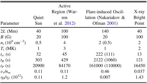
In the rest of this paper we discuss wave heating for a series of loop parameters summarized in Table1. The lengths, plasma parameters, and magneticfield strengths(rows 1–4)correspond to(1) short loops, perhaps in the quiet Sun;(2)typical active region values (e.g., Warren et al. 2012); (3) the long (fl are-induced) oscillating loops originally identified by Nakariakov et al. (1999); and (4) small structures such as X-ray bright points. (Bracketed quantities for case 3 are discussed in Section 3.2.)

The damping of standing shear Alfvén waves by phase mixing was discussed byHP83and Browning & Priest(1984)

for Cartesian geometry. The wave is confined to oscillate between two photospheric boundaries of a magnetically closed structure such as a coronal loop of total length 2L. The loop axis is assumed to lie in the z-direction along the background magneticfield, the wave magnetic and velocity components are in they-direction, and the density gradient is in thex-direction. Under these conditions, the Alfvén wave is damped (and dissipated)according to(e.g.,HP83, Browning & Priest1984)

( )= ( ) [ (- ( )) ] ( ∣∣ ) W( ) ( )

v x ty , v xy , 0 exp t tP x 3 sin k z sin x t 1

with k =p 2L to represent a standing wave. The magnetic

field follows from Faradayʼs law, and the characteristic damping time for phase mixing is

( [n ] ) ( )

= W

tP 36 d dx2 2

with n=nm+nv, the sum of the resistive and viscous damping coefficients (see the Appendix for a discussion of these),W =pqV xA( ) 2 ,L q the mode number,Lthe loop

half-length (we will use this definition throughout the paper), and for a uniform magnetic field dΩ/dx = −Ω(dρ/dx)/2ρ. Note thatq=1 corresponds to a mode with wavelength 4L(referred to as the global mode). For “classical” transport, tP is large

(Table1, row 7 and theAppendix), typically tens of thousands of seconds or more.(In Table1, plasma quantities are defined as being in the high-density region.)

For resonant absorption we consider the straight field case for the well-studied cylindrical loop geometry. If there is a smooth density profile linking high- and low-density regions (ρiand ρe, respectively)through a layer of widthl, the global mode feeds energy into the layer at an approximate rate(e.g., Goossens et al.1992; Ruderman & Roberts2002):

( )

( ) ( )

p r r r r

= +

-t a

l t

2 1

1 3

R i e

i e W

where a is the transverse scale of the global oscillation (typically assumed to be a loop radius so thata/Lis roughly the aspect ratio of the loop) and tW~23 2L(1+r re i) VA

1 2 _is

the period of the global mode (Nakariakov et al. 1999; Ruderman & Roberts2002), with the Alfvén speed determined by ρi. The wavelength of this global (fundamental) mode is twice the loop length.3Typical values oftWandtRforρi?ρe

anda/l=10 are given in Table1, rows 5 and 6. The damping times lie between 100 and 2000 s, with the largest value for the longest loops. Shorter damping times, as suggested by Nakariakov et al. (1999) and Nakariakov & Ofman (2001) for long loops, can be obtained by adjusting the parameters.

Note that the expressions for tWand tR (Equation(3))give

the period and damping time for the resonantly damped, fundamental (radial) mode of a thin flux tube. While such a single-frequency driver has one resonant layer, a broadband spectrum may have multiple resonant layers, all within the widthl(e.g., De Groof & Goossens2002). The results in our paper apply to the scenario of a single,fixed frequency. For a broadband driver, the situation may well be somewhat different; although the supporting plasma structure may be

Table 1

A Range of Loop Parameters, Damping and Dissipation Times and Associated Quantities

Parameter

Quiet Sun

Active Region(

War-ren et al.2012)

Flare-induced Oscil-lation(Nakariakov &

Ofman2001)

X-ray Bright Point

2L(Mm) 40 100 140 40

B(G) 20 100 20 100

ni(109cm−3) 0.5 4 2(0.5) 2

Ti(MK) 1 3 1 2

tw(s) 32 45 222(111) 13

tR(s) 303 429 2122(1060) 121

tP(s) 20900 84170 161000(110000) 16450

νv/nm 0.11 0.11 0.46 0.037

η0/η1(1012_{) 0.11 1.2 0.007 1.43}

Note.For case 3, we use two densities, as discussed in the text.

3

changing, resonant absorption will continue to occur, although likely at varying positions.

Although using different geometries, both of the above examples illustrate wave-based heating underpinned by a local density gradient. Finally, we point out that we are equating the wave-damping time due to phase mixing or resonant absorption with the timescale for plasma heating. This can be considered to be a best-case scenario, in the sense that clearly no (wave) heating can occur before(substantial)wave damping occurs. If there is a lag between the wave damping and the actual plasma heating, the conclusions of Section3 will be strengthened.

3. THE RELATION BETWEEN WAVE DAMPING AND DENSITY STRUCTURES

In most models of wave damping due to phase mixing and resonant absorption, a stationary density gradient is imposed, although slowly varying densities are also now being considered in some problems (e.g., Morton et al. 2010; Williamson & Erdelyi 2014a, 2014b). However, it was noted in the introduction that any density structuring in the closed corona is associated with variable levels of coronal heating. This section asks whether these imposed density gradients are consistent with the energy deposited owing to wave heating, as well as how a temporally evolving(transverse)density profile changes the nature of wave damping. We again emphasize that we are addressing this from the point of view of an initial value problem where a density gradient is assumed to exist and waves are injected into it.

3.1. Are Assumed Density Structures Compatible with Wave Heating?

As a simple example, consider steady heating. In this case, well-known scaling laws (e.g., Craig et al. 1978; Hood & Priest1979)lead to the following relations between the coronal plasma and heating per unit volume (H)4:

( )

( ) ( )

~ ~ - a ~ - a - a

T7 2 HL2, nL T 7 2 4, n H7 2 14L 2 7 4

where a radiative loss L( )T =cTa is assumed (see, e.g., Klimchuk et al. 2008). Typical values lie between−1/2 and −3/2; for the former arises the familiar result T~n1 2_{, and}

unless otherwise stated, we assumeα=−1 andχ=4×10−16 in cgs units. Thus, a high-density region requires more heating if it is to be in static equilibrium.

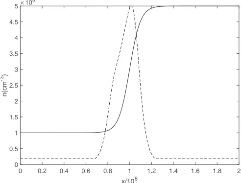
For the density profiles used in contemporary calculations of resonant absorption and phase mixing, heating is focused either at the resonance layer or in the vicinity of the point of maximum density gradient, respectively, rather than in the high-density regions. Figure1shows some of the consequences of this in a simple example of phase mixing. The basic parameters are as in case 1 of Table1, although the results are generic. Throughout the paper we assume an initial density profile of the form (solid line in Figure1)

( )= [ +( )( + {( - ) }] ( )

n x n0 1 f 2 1 tanh x x1 xsc 5

and setn0=10 8

cm−3,f=4,x1=10 8

cm,xsc=10 7

cm, and

L= 2×109cm. For the case of phase mixing, which we now discuss, the wave propagates in the z-direction, with magnetic

field and velocity perturbations in the y-direction. Note also that locally the density profile in a thin layer is independent of whether this layer forms the boundary in a Cartesian or a cylindrical system, and hence we can also use the same density profile(Equation(5))for resonant absorption, as in Section3.2. We now use Equations(1) and (2)to calculate the heating associated with phase mixing in the density profile (5). Equation (1) is averaged over a wave period and the loop length, so that the decrease in wave kinetic energy as a function of time is then 1 2r( )x vá y0( )x ñ2[1-exp[-2(t t xp( )) ]]3 , where á ñvy0 denotes the averaged initial velocity. For this

example, we use an initial averaged wave amplitude of 30 km s−1, but the result is generic. Since a shear Alfvén wave has equal kinetic and magnetic energy, the wave energy

(kinetic+magnetic) lost over time is

( ) ( ) ( ) [ [ ( ( )) ]]

dEw x t, =r x vá y0 x ñ2 1-exp -2 t t xp 3 , which in

turn determines a heating rate. To calculate H for use in Equation (4),we sum δEw over 2 minutes (tP) to obtain an

average heating rate. (Note that the diffusion is enhanced by 106in order to give damping times of interest; see Section4.1 and the Appendix.) The density associated with this heating then follows from the scaling laws(4) (dashed line in Figure1). (Note that in order to avoidT and n becoming zero, a weak constant background heating is imposed, which is added to the wave heating. This background heating is taken to be 10−2H(x

= 0), as given by Equation (4).) Clearly, the two density profiles differ considerably (note that the two profiles have been normalized to their respective maxima). The new density profile requires a mass flow to and from the chromosphere along the magnetic field, as discussed by, for example, Antiochos & Sturrock (1978) and Klimchuk et al. (2008). The flow is of order 15–30 km s−1depending on the specific situation. A similar conclusion would hold for resonant absorption (when considering a single-frequency driver): the heating at the resonant layer(for example, halfway through the density gradient)will give a density spike there, while the rest of the loop is unheated (e.g., Ofman et al. 1998). Thus, the initial imposed density profile is incompatible with the density implied by the wave heating.

Figure 1.Initial imposed density(solid line)and density calculated in response to the heating(dashed)for phase mixing, where the density is calculated from static loop scaling laws(Equation(4)). The heating is the sum of a low-level background and the heating due to phase mixing averaged over 2tP.

4

3.2. Temporal Evolution of an Imposed Density Structure

Equation(4)is limited in its assumption of an instantaneous adjustment of the density to the wave heating. In reality, a loop would not evolve immediately from one density structure to another, and it is important to see how the temporal development of the density structure can impact wave damping. We discuss the evolution of a prescribed density profile using the Enthalpy Based Thermal Evolution of Loops (EBTEL)approach(Klimchuk et al.2008; Cargill et al.2012a,

2012b, 2015), an approximate zero-dimensional model that

treats the corona and transition region(TR)as separate entities, matched at the boundary between them. Assuming symmetry about the loop apex, the coronal density and pressure evolve according to

( )

( )

( ) ( )

g

g g

- = - + +

= = - - +

dp

dt L R R H

dn dt

nv

L kT L F R

1 1

1

,

1

2 6

c

c tr

0

0

0 tr

wherep,n, andTare coronal averages, taken to be the same as the assumed(uniform)plasma distribution along the loop axis used in wave calculations. Fc0= -(2 7)k0Ta7 2 L is the heat flux at the top of the TR,Rc»n2L( )T Lthe integrated coronal

radiation,Rtrthe integrated TR radiation, subscript“0”denotes

a quantity at the top of the TR, and subscript“a”a quantity at the loop apex. The temperature follows from the equation of state. Solving this set of equations requires the specification of three (semi-)constants that are defined as C1 = Rtr Rc,

=

C2 T Ta, and C3=T T0 a, as discussed fully in Klimchuk

et al.(2008)and Cargill et al.(2012a).C2andC3can be taken

as constant, with values of 0.9 and 0.6, respectively. C1is, in

the absence of gravity, 2 for equilibrium, static loops and 0.6 during radiative cooling.

The study has two parts. First, we examine how the facilitators of damping, a density gradient in the case of phase mixing and the location of the resonant layer for resonance absorption, change as an imposed density structure [n(x)]

evolves in the absence of heating. For current wave-heating models to be valid, the density structure must remain approximately unchanged over the time required for wave damping to become effective. In Section 4 we discuss how heating might operate in such an evolving density structure.

Consider a loop that is in equilibrium according to Equation (4)and switch off the heating. This models the situation in the usual initial value problem where a coronal density structure is imposed, and waves are then introduced into the plasma. In the absence of any wave heating, the loop cools and drains through four phases: (i)first conduction and radiation both contribute, but, as the temperature falls, (ii)radiation becomes dominant with T ∼n2. This phase is characterized by a slow subsonic downflow whose associated enthalpy flux powers the TR radiation (e.g., Reale et al. 1993; Bradshaw & Cargill 2010). Cargill & Bradshaw(2013)argued that at a critical temperature of order 1 MK for short loops, this phase breaks down and phase(iii)begins, characterized by a rapid temperature fall with a slowly varying density. The onset is determined by the inability of sound waves to sustain a subsonic flow as the temperature falls. During this phase, the corona becomes more overdense, so it cannot be sustained in hydrostatic equilibrium, and in phase (iv) it drains rapidly. Although it is the density

structure that is important for wave damping and/or dissipa-tion, the temperature evolution is also of importance for the onset of phase (iii). We will be mainly concerned with the duration of phase(ii).

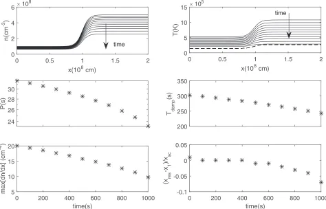
We again(locally)consider the boundary density profile as given by Equation (5), so that there is a density change of a factor offive going from left to right(see Figure1). We again stress that the cooling calculation is independent of whether the loop boundary is a slab or a cylinder. Two sets of initial conditions for the temperature are considered: one where the temperature is assumed to be constant with the value given in Table 1 (Figure 2), and a second where it is related to the density through Equation(4) (Figure3). The EBTEL approach allows us to study spatially well-resolved transverse density structures quickly. Equations(6)are solved at 2000 points in thex-direction for 1000 s. This takes a few minutes on a laptop. The results for cases 1, 2, and 4 (see Table 1) are quantitatively similar, so only case 1 is shown. Case 3 is discussed separately. In Figures2and3, the top row shows the evolution of the density and temperature as a function of time. The dashed line in the right panel is the critical temperature for the onset of catastrophic cooling (Equation (5) of Cargill & Bradshaw2013). The curves are plotted every 100 s, with both

Tandndecreasing with time. The two plots in the second row show the period of the global mode(left)and the damping time (right) from Ruderman & Roberts (2002) and Section 2, assuming that these quantities can adjust to the evolution of the density. In practice, this is done by calculatingρeandρifrom the hydrodynamic EBTEL model(Equation(6))and substitut-ing these into the expressions for tW and tR from Section 2.

(Note that the damping times for phase mixing, as given by Equation (2), would generally be considerably longer but would qualitatively show similar behavior.)The last row shows the maximum value of the density gradient (left) and the location of the resonant point with respect to its initial value (x1), which is located at the midpoint of the density gradient

(right). The latter is calculated by noting that the resonant condition is given by 4L =t Bw z 4pr(x=xres), using the updated expression for tw to evaluate ρ(x=xres), and finally

solving forxresfrom the hydrodynamic calculation of ρ.

The two initial conditions give different results. When the initial temperature is assumed to be constant, the high-density region of the loop cools rapidly, the period of the wave (damping time) decreases (increases) owing to the smaller density (density jump), the resonance point expressed as the ratio(xres–x1)/xsc moves to the left by approximately 0.4xsc,

and the maximum density gradient also falls and its location moves to the left. When the temperature and density are everywhere related by Equation (4), the period of the wave falls, but the damping time also decreases such that their ratio remains nearly constant. The resonance point stays almost exactly at its original location(note the very different scales on they-axis of the bottom right panel of Figures2 and3), while the maximum density gradient falls, although its location also does not move. For this case xsc = 180 km, but the

dimensionless quantity (xres–x1)/xsc is roughly independent

ofxsc.

Figure 2.Evolution of the average density and temperature profiles over 1000 s. Loop parameters for case 1 are used, and the initial temperature is constant. The top row shows the density(left)and temperature(right)every 100 s. The dashed line is the condition required for the onset of phase(iii)of the loop cooling(see text). The middle row shows the wave period(left)and damping time(right)as a function of time. The bottom row shows the maximum density gradient(left)and position of resonance layer(right)as a function of time.

s−1, which leads totdrainof order 1000 s, consistent with these

results. To understand the motion of the resonance layer and the location of the maximum density gradient, we use the fact that a loop cooling by radiation satisfies approximately(Cargill et al.1995)

( ) ( )

t

= ⎡

-⎣⎢

⎤ ⎦⎥

T t T 0 1 A t R

B

0

where A and B are constants that can be assumed to be independent of the plasma conditions (see the Appendices of Cargill et al. 1995 and Cargill 2014 for details) and

( )

tR0=3kT n R T0 0 L 0 , the radiative cooling time at t=0. For

a constant initial temperature, tR0(x) ∼ 1/n0(x), so that the

right-hand side of the loop (higher density) in Figure 2 will cool faster. For a loop in initial static equilibrium at all values ofx, the second equation of Equation(4)can be used to relate

n0and T0 asn0(x)∼ T0(x)(7/4–α/2), so thattR0(x) ∼ T0(x)−(3/ 4+α/2)_{, a weak dependence onT0. This initial state ensures that}

the cooling time (and hence the draining time) is weakly dependent onx,meaning that the density structure is preserved as the loop cools, with the resonance point remaining at the same location.(For the caseα=−3/2 we have confirmed that there is no movement at all inxres.)The behavior of the wave

period and damping time follow. The period will always fall because the density falls. For the constant-temperature initial conditions, the density gradient across the resonance layer decreases (right side drains faster), so that the damping time increases. For the static loop initial state, the ratioρi/ρeremains roughly constant as the loop drains, so that the damping time also decreases.5

Thus, for initial conditions corresponding to static equili-brium atmospheres, energy may continue to enter a fixed resonant layer of a cooling loop despite the continually evolving loop density. For other initial states, the resonant layer moves, making it less clear whether wave damping can occur. For phase mixing, the density gradient persists throughout the cooling and draining, though with diminishing values. Since the damping time depends on the density gradient to the power 2/3, damping may become weaker as time increases, accentuating the difficulties with the (slow) rate of heating in phase mixing.

To assume a fixed density profile in wave calculations, the damping time(dissipation time)for resonant absorption(phase mixing)must be shorter than the draining time if the resonance layer (location of maximum density gradient)does not move, or less than the characteristic time over which these quantities move. Violation leads to the termination of heating because the coronal density structure needed for wave heating is destroyed. Row 7 of Table 1 shows that for phase mixing a large enhancement of the transport coefficients is required, an assumption prevalent in the literature(Appendix). For resonant absorption, these conditions may be met for short loops and/or

strong magneticfields, but significantly not for the long loops for which resonant damping is frequently invoked (e.g., Goossens et al.2006, 2011). The viability of a fixed density profile must thus be assessed on a case-by-case basis.

4. CONSEQUENCES OF EVOLVING DENSITY FOR WAVE HEATING

If wave heating cannot sustain the initially imposed density profile, what happens? A simple calculation for resonant absorption was due to Ofman et al. (1998),6 who studied a linear initial value problem and included the feedback of an evolving density profile using Equation (4), which fed an updated density into the wave-damping calculation. This evolving density led to a “detuning” of the resonance from its initial location, with the heating moving to elsewhere in the loop. Starting with a smooth density profile with asymptotic values differing by a factor of 10, the density evolved into a spiky structure(Figures 3–5 of Ofman et al.1998). The initial density profile could not be sustained, and the time-averaged density fell to roughly 20% of the initial value. Thus, in this case there was a mismatch between the energy injected and the initial density (and associated thermal energy), the former being too small. This could presumably have been mitigated by an increase in the incoming wave power. For the case of a single driver frequency, total detuning took place, with no heating, the loop drained of all material, and resonant conditions could not be recovered.

4.1. General Considerations

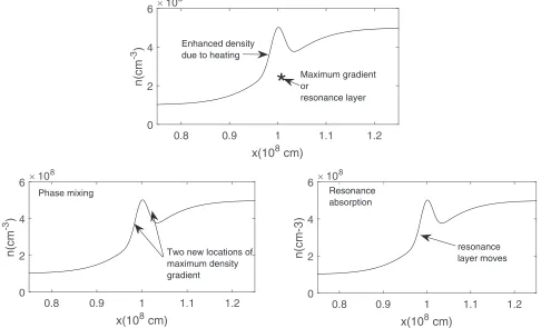
The assumption of an instantaneous adjustment to static equilibrium by Ofman et al. almost certainly overestimates the rate at which standard resonant absorption breaks down. We have shown in Section3that the detuning that may take place can be relatively slow. Although time-dependent simulations of an Ofman-like scenario seem desirable, one can make some simple generic comments. Figure 4 shows in a schematic manner some of the issues for resonant absorption and phase mixing(see also Figure 4 of Klimchuk2006).

The initial density profile is the smooth solid line and increases from left to right. For convenience we locate the resonant layer and location of steepest gradient in the middle, and it is there that the heating is strongest(star symbol in the diagram). The heating leads to a density enhancement, as shown. For phase mixing, this density spike can have two points of enhanced dissipation, one on either side of the new density maximum(lower left panel). Heating at these may then lead to two new density spikes, etc., and one can see that a runaway process with a very spiky density could arise, potentially leading to fast wave dissipation. For resonant absorption, the simplest scenario is for the location of the resonant layer to move as shown, so that the resonant frequency matches the new density profile, a less drastic process than that discussed in Ofman et al. However, we note that more structured multipeaked density profiles may lead to a more complicated situation. Although a full, explicit model of this scenario would, in general, require MHD simulations that couple thermal and MHD evolution, we present a simple

5

Case 3 with a constant temperature is the exception to these results. Wefirst considered values ofTandn(1 MK and 2×109cm−3, respectively)used in the analysis of transverse oscillations(e.g., Nakariakov & Ofman2001; White & Verwichte2012). In this case, the loop enters phase(iii)of the cooling almost immediately, and the density structure ceases to exist after 200 s. It seems that these commonly used plasma parameters may not be appropriate as such a loop does not appear sustainable on relevant timescales(unless an additional heating mechanism is operating). Adoption of a smaller density as shown in the bracketed terms in Table1recovers the generic results of cases 1, 2, and 4.

6

example in the next subsection to demonstrate the basic concept.

4.2. Heating by Phase Mixing in an Evolving Atmosphere and the Role of Feedback

Next, we consider heating by phase mixing in the evolving atmosphere discussed in Section 3. The case of resonant absorption will be discussed in a subsequent publication. The decrease in wave energy (kinetic +magnetic)from an initial state and averaged along the loop is dEw(x t, ) as defined in Section 3.1, and the heating rate follows. Table 1 shows that with classical coefficients, tpis much longer than the cooling

time, so for phase mixing to be viable,vmust be enhanced by several orders of magnitude. As in Section 3.1, for case 1, our main example here, an increase of six orders of magnitude is used. This enhancement is discussed further in the Appendix, and the dependency of v on density and temperature is neglected since any anomalous diffusion is unlikely to have the same scalings as classical. Also, to simulate a driven system, the wave amplitude is re-initialized every 25 s, which is of order the wave period. This models an effective Poyntingflux through the photosphere. For case 1, the wave amplitude after each re-initialization, averaged over the loop length and a wave period, is approximately 30 km s−1. Cases 2–4 are discussed later.

Figure5 shows results for case 1. Thefirst example has an energy equation where radiative and conductive losses are ignored, implying a background heating that sustains the initial density profile. Since the wave heating only determines the change in pressure, there is freedom to apportion this pressure

change between density and temperature. First, we adopt a scaling T ∼ nb, where b =0 corresponds to no temperature change,b =1/2 to a static loop scaling(see Section3), and

b = 2 to a loop where the temperature is determined by radiation (Bradshaw & Cargill2010). The top row shows the density and temperature after 1600 s. The solid, dashed, and dot-dashed lines haveb=0, 1/2, and 2, respectively, and the thick dashed line in the right panel is the heating in arbitrary units averaged over the 200 s before the end of the run. A new density peak appears, and the heating spreads away from the center of the density gradient, similar to what was shown in Figure1. The maximum of the heating is displaced to the high-density side because of the dependence onnof the wave kinetic energy, but the maximum of the heating per unit density (not shown) is roughly located at the location of the maximum density gradient. Note, however, that the new density peak is also displaced to the higher-density side of the density gradient. As is expected, larger values of b have weaker density enhancements.

The second row shows the density and temperature at 1600 s using the EBTEL approach described in Section 3.2 (solid lines)and the static scaling laws(dashed lines). For the EBTEL calculation the heating is the same as in the upper row, and for the scaling law the heating is averaged over consecutive 200 s intervals, and then the scaling laws are applied. The density in the heated region is similar for both models, but to the left and right it decreases since there is no heating to support the plasma (see Figure1). When the scaling laws are used, this decline is instantaneous. This confirms the suggestion made at the start of Section 3 that the prescribed density profiles used in such

calculations are unsustainable: the density evolves from a step between a low and a high value to a localized peak.

Inclusion of feedback of the new density profile on the wave heating requires an MHD simulation that could be restricted to the linearized wave equations plus an energy equation. However, for demonstration purposes we have carried out a simple model to include density feedback using the following procedure. EverytNseconds, the density in the wave-damping

calculation (1) is reset to the new value calculated from the energy equation and the model restarted. However, we found that this could lead to discontinuities in the damping time and hence spuriously enhanced damping, since changing the new density gradient, when folded in with the previous time, implies that the phase mixing is more developed than it should be. Instead, when the density is reset, we force the damping time to be continuous. This is done by re-defining the“time” associated with eachfield line such that the quantityt*/tp(x)is the same before and after the density reset, wheret*is a dummy time: when we reset the density, we definetp(old)andtp(new)

as the damping times associated with the old and new density profiles and then set t* = t_* (tp(new)/tp(old)) such that the

factor _e-t tp(old) _=e-t tp new( )_{. Thus, if the density gradient}

steepens(lessens),tpdecreases(increases)and hencet*at that

location is decreased(increased). This process is repeated every time the density is reset, and it is nothing but a straightforward bookkeeping exercise to ensure that the damping time remains continuous.7

The results are shown in Figure6, which has a compressed

x-axis and enhancedy-axis to show the important features. We have run feedback in both models withtN=200 s: without(left

panel)and with(right panel)full energetics. For the former, we

see small density spikes beginning to appear near the center of the density gradient, which on subsequent iterations develop rapidly. Within a few iterations these are at grid size. With the EBTEL solution, spikes again develop, but they are much more muted: the loop thermal evolution is too important for the feedback to have a real effect in this case.

Cases 2–4 have also been examined. To permit a comparison with case 1, we have reset the dissipation coefficients and wave amplitude so that the temporal evolution is similar to case 1. Explicitly, this means that we require that the peak density take on similar values after 1600 s to that shown in Figure5and that

tpis also the same. This requires an increase of the diffusion by

a factor of 10 for cases 2 and 3 and a decrease by a factor of 0.4 with case 4. For cases with no feedback, the averaged wave amplitude was increased by 1.75 for case 2, by 1.5 for case 4, and remained the same for case 3. We then ran these cases with feedback. In the absence of a full energy equation, results similar to the left panel of Figure 6 were obtained. With the EBTEL approach, case 4 was similar to case 1, but cases 2 and 3 took longer (2000 and 3000 s, respectively) to reach the equivalent density structure.

5. CONCLUSIONS

MHD wave-heating mechanisms such as phase mixing and resonant absorption crucially depend on a local density gradient. However, few, if any, studies have examined MHD wave heating in the context of an evolving density gradient, and it is not a priori clear whether the density gradient required for dissipation is compatible and/or sustainable by the wave-heating mechanism. This paper has addressed two aspects of this question. We have presented a proof of concept that (i) such density profiles may not be sustained because the density gradients are destroyed by plasma cooling on a timescale compatible with or faster than the heating, which in turn implies that(ii)the density profiles assumed in models of wave dissipation may be incompatible with the spatial distribution of the heating. When such cooling and draining take place, the movement of the dissipation layer depends on the chosen initial

Figure 5.Density and temperature after 1600 s for wave damping by phase mixing. The upper two panels show cases when there are no radiative or conductive losses. The solid, dashed, and dot-dashed lines show cases whereT∼nb_{, withb=0, 1/2, and 2, respectively. The lower dotted lines are the initial density and temperature,}

and the temperature forb=0 is not shown since it is unchanged from the initial state. The thick solid line in the right panel is the wave heating in arbitrary units. The lower panels include an energy equation. The solid line shows results using EBTEL, and the dashed line results using a static loop scaling law, with the dotted line showing the initial conditions.

7

conditions. Incorporation of feedback can, in principle, lead to highly structured density profiles for both resonant absorption and phase mixing, but in reality the timescale for this to evolve is comparable to the time taken for a loop to cool and drain, and hence it may only play a small role. Thus, the temporal evolution of the plasma in which any wave heating takes place seems to be an essential factor in considering the viability of wave-damping mechanisms. One option is that an alternative heating mechanism such as small-scale reconnection can maintain the required density profile, and wave damping can then take place as proposed in the literature.

It is worth pointing out that the restrictions we have noted for wave heating do not apply to mechanisms for coronal heating that rely on small-scale reconnection, commonly referred to as “nanoflare heating.” Here all that is required is the misalign-ment of the coronal magneticfield to a degree that permits the onset of reconnection. While the form this takes remains an open question, it is commonly assumed that the local plasma density structure plays no role. Studies of reconnection where a density gradient is present are common in studies of the terrestrial magnetopause(Levy et al.1964)and summarized by Lin & Lee (1993). There are qualitative changes in quantities such as reconnection rates, but the overall generic properties of reconnection are unchanged.

While this paper has only addressed simple examples of wave heating, the conclusions are general. In particular, extensions to broader density transitions (e.g., Soler et al.2013), the injection of an Alfvén continuum(e.g., Poedts et al. 1989), and examples of complexities in the damping process (e.g., Poedts & Boynton1996)will undergo the same form of generic feedback of the density. Similar conclusions apply to wave dissipation in force-free fields with initially constant density(e.g., Poedts et al.1989). In that case, heating at a resonant layer with either a single wave frequency or a continuum will lead to plasma heating, a subsequent change in the density, and a modification of the resonant conditions. Understanding the full consequences will require numerical modeling, but the basic physical process outlined here is expected to occur regardless of additional complexities.

Examination of phase mixing in this environment brings long-standing problems into fresh focus. For classical transport coefficients, the fundamental difficulty is the slow dissipation of the wave energy; we were unable to find cases where the

damping time was short enough to be of interest. Further, ways that phase mixing could give faster damping, such as the density feedback discussed here and the development of compressive waves (e.g., Nakariakov et al. 1997, 1998; Tsiklauri et al.2001; McLaughlin et al.2011), cannot happen until the phase mixing itself becomes well developed, a slow process. Other mechanisms such as the Kelvin–Helmholtz instability(Browning & Priest1984; Antolin et al.2014)may be promising, but require more investigation. In order to demonstrate the interaction of loop plasma evolution with wave damping, we have argued that the transport coefficients are enhanced artificially by an unspecified process. A more pessimistic view may be that for closed coronal structures, phase mixing is unviable.

Verification of our conclusions will in general require multidimensional MHD simulations, which will be quite challenging given the competing constraints of the small time step needed for numerical stability and the long times that need to be run. Only then can a definitive answer be reached as to the viability of coronal wave-damping processes, although our work suggests that caution is warranted.

We thank Alan Hood for several helpful discussions. This project has received funding from the Science and Technology Facilities Council (UK) and the European Research Council (ERC)under the European Unionʼs Horizon 2020 research and innovation program (grant agreement No 647214). The research leading to these results has also received funding from the European Commission Seventh Framework Pro-gramme (FP7/2007-2013) under the grant agreement SOL-SPANET(project No. 269299,www.solspanet.eu/about).

APPENDIX

TRANSPORT COEFFICIENTS AND PHASE MIXING

In their paper on phase mixing, HP83 used classical resistivity and viscosity coefficients. The Braginskii (1965) viscosity has five terms, three of which are associated with compressive effects. Defining the ion–ion collision time as

ti=0.84T3 2 n, the compressive (kinematic) viscosity is

( )

h r0 =0.96 kT mi ti=6.46´107T5 2 n, agreeing with

HP83, Equation (22). To calculate the shear viscosity,

as modified by the magnetic field, η0 is reduced by a factor of 1/(τiΩi)2, or 1.4×10−8n2/B2T3, to give

nv=h1/r=0.9n B T2 1 2 (correcting the viscous term

tem-perature dependence in HP83).8 This is the viscosity used in Equation (2). The resistive damping term is nm=1013 T3 2.

The ratio of shear viscous damping to resistive damping is then 9×10−14nT/B2=13β, whereβ=8πp B−2, and is shown in the 8th row of Table1. For all our parameters resistive damping is the more important, and in three cases it is dominant. The ratio of shear to compressive viscosity is shown in thefinal row of Table 1, so any process that introduces a compressive component may be important.

The damping times due to phase mixing (tp) are given in

Table 1. One can write Equation (2) as

[ p ] n

=

tp 3 6 4LLx qVA 2 , where L is the total loop length,Lx

the length over which the density changes, and q the mode number. Thus, short loops, high harmonics, and sharp gradients are optimal, but on taking Lx ∼ 200 km, tp is always rather

large, as is the ratio tp/tw; we see no reasonable likelihood of finding the values of 20 quoted byHP83for this ratio.(Note that for only viscous damping,tp=6.1 10-83 (L L2 x2 q T2) 1 2, independent ofBand n.)

As we have noted, to obtain damping times of order or less than a cooling time, the transport coefficient needs to be increased by many orders of magnitude. One way to do this would be to invoke nonlinear MHD effects such as a coupling to the fast- or slow-mode waves that introduce a compressive viscosity. The compressive waves would damp, in turn, at a rate inversely proportional to the Reynolds number calculated using compressive viscosity, with a damping time

r h

~

tc Lc2 0, where Lc is a compressive wave scale. The

ratio of the damping times istp tc~3.93 [LLx q T]2 8 3 nLc2,

and for Lc ∼ 10 9

, these can be comparable. Thus, the 1/3 dependence of the phase mixing compensates for the weak transverse viscosity. In addition, nonlinear effects are unlikely to develop before phase mixing is well under way, so invoking compressive viscosity actually gains very little since the longevity oftpis due to the long time before the phase mixing

becomes strong enough to lead to nonlinear effects.

There are two common solutions to these long dissipation times. One just invokes an ad hoc enhanced dissipation, as is done in many numerical calculations. For example, McLaugh-lin et al.(2011)define a dimensionless viscosityνsc=L0VA0.

For our parameters, this is 1.38 1014cm2s−1. A dimensionless viscosity of 10−2such as they use implies a viscosity 108times larger than given by classical models. On the other hand, Browning & Priest (1984) argue for a massive (unspecified) enhancement due to a local Kelvin–Helmholz instability. At the antinode of the standing wave the velocity gradients are strongest while the perturbedfield vanishes, and the latter effect reduced any (stabilizing)magnetic tension forces have on the instability. This analysis requires that the instability grow faster than the period of the wave, so that it can be assumed that the antinode constitutes an equilibrium. Browning and Priest examine two cases: strong and weak phase mixing. Based on their results, we can write down a simple expression for the

kinematic viscosity: n ~10-2Va_{, where a is the transverse}

scale of the density gradient andVis the wave amplitude. This gives a viscosity of 4×1012cm2s−1for a wave amplitude of 40 km s−1 and a shear width of 108cm, hence 8–9 orders of magnitude larger than the classical shear value. In turn, this reduces the damping time from 30,000 s to about 100 s. Further investigations are required to assess the viability of this mechanism.

REFERENCES

Antiochos, S. K., & Sturrock, P. A. 1978,ApJ,220, 1137

Antolin, P., Yokoyama, T., & Van Doorsselaere, T. 2014,ApJL,787, L22 Arregui, I, 2015,RSPTA,373, 20140261

Belien, A. J. C., Martens, P. C. H., & Keppens, R. 1999,ApJ,526, 478 Bradshaw, S. J., & Cargill, P. J. 2010,ApJ,717, 163

Braginskii, S. I. 1965, RvPP,1, 205

Browning, P. K., & Priest, E. R. 1984, A&A,131, 283 Cargill, P. J. 2014,ApJ,784, 49

Cargill, P. J., & Bradshaw, S. J. 2013,ApJ,772, 40

Cargill, P. J., Bradshaw, S. J., & Klimchuk, J. A. 2012a,ApJ,752, 161 Cargill, P. J., Bradshaw, S. J., & Klimchuk, J. A. 2012b,ApJ,758, 5 Cargill, P. J., Mariska, J. T., & Antiochos, S. K. 1995,ApJ,439, 1034 Cargill, P. J., Warren, H. P., & Bradshaw, S. J. 2015,RSPTA, 373, 201400260 Craig, I. J. D., McClymont, A. N., & Underwood, J. H. 1978, A&A,70, 1 De Groof, A., & Goossens, M. 2002,A&A,386, 691

De Moortel, I., & Nakariakov, V. M. 2012,RSPTA,370, 3193 Goossens, M., Andries, J., & Arregui, I. 2006,RSPTA,364, 433 Goossens, M., Erdélyi, R., & Ruderman, M. S. 2011,SSRv,158, 289 Goossens, M., Hollweg, J. V., & Sakurai, T. 1992,SoPh,138, 233 Heyvaerts, J., & Priest, E. R. 1983, A&A,117, 220(HP83) Hood, A. W., & Priest, E. R. 1979, A&A,77, 233 Ionson, J. A. 1978,ApJ,226, 650

Klimchuk, J. A. 2006,SoPh,234, 41

Klimchuk, J. A., Patsourakos, S., & Cargill, P. J. 2008,ApJ,682, 1351 Lee, M. A., & Roberts, B. 1986,ApJ,301, 430

Levy, R. H., Petschek, H. E., & Siscoe, G. 1964,AIAAJ,2, 2065 Lin, Y., & Lee, L. C. 1993,SSRv,65, 59

Martens, P. C. H. 2010,ApJ,714, 1290

McLaughlin, J., de Moortel, I., & Hood, A. W. 2011,A&A,527, A149 Morton, R. J., Hood, A. W., & Erdelyi, R. 2010,A&A,512, A23 Nakariakov, V. M., & Ofman, L. 2001,A&A,372, L53

Nakariakov, V. M., Ofman, L., DeLuca, E. E., Roberts, B., & Davila, J. M. 1999,Sci,285, 862

Nakariakov, V. M., Roberts, B., & Murawski, K. 1997,Sol Phys,175, 93 Nakariakov, V. M., Roberts, B., & Murawski, K. 1998, A&A,332, 79 Nakariakov, V. M., & Verwichte, E. 2005, LRSP,2, 3

Ofman, L., Davila, J. M., & Steinolfson, R. S. 1994,ApJ,421, 360 Ofman, L., Davila, J. M., & Steinolfson, R. S. 1995,ApJ,444, 471 Ofman, L., Klimchuk, J. A., & Davila, J. M. 1998,ApJ,493, 474 Parker, E. N. 1991,ApJ,376, 355

Poedts, S., & Boynton, G. C. 1996, A&A,306, 610 Poedts, S., Goosens, M., & Kerner, W. 1989,SoPh,123, 83 Poedts, S., Goosens, M., & Kerner, W. 1990,ApJ,360, 279 Rae, I. C., & Roberts, B. 1981,GApFD,18, 197

Reale, F. 2014,LRSP,11, 4

Reale, F., & Landi, E. 2012,A&A,543, A90 Reale, F., Serio, S., & Peres, G. 1993, A&A,272, 486 Ruderman, M. S., & Roberts, B. 2002,ApJ,577, 475

Soler, R., Goossens, M., Terradas, J, & Oliver, R. 2013,ApJ,777, 158 Tataronis, J. A., & Grossman, W. 1973,ZPhy,261, 203

Tsiklauri, D., Arber, T. D., & Nakariakov, V. M. 2001,A&A,379, 1098 Warren, H. P., Winebarger, A. R., & Brooks, D. H. 2012,ApJ,759, 141 White, R. S., & Verwichte, E. 2012,A&A,537, A49

Williamson, A., & Erdelyi, R. 2014a,SoPh,289, 899 Williamson, A., & Erdelyi, R. 2014b,SoPh,289, 4104

8

TheHP83analysis seems to contain a few numerical errors and typos. They

find1 (tiW =i) 3.510-4n BT3 2, so that the correction(the square)is 1.23