Type 2 fuzzy linear systems

(will be inserted by the editor)

Type-2 Fuzzy Linear Systems

Marzieh Najariyan · Mehran Mazandarani · Robert John

Received: 04.08.2016 / Accepted: 27.12.2016

Abstract Fuzzy Linear Systems (FLSs) are used in practical situations where some of the systems parameters or variables are uncertain. To date, in-vestigations conducted on FLSs are restricted to those in which the uncertainty is assumed to be modeled by Type-1 Fuzzy Sets (T1FSs). However, there are many situations where considering the uncertainty as T1FSs may not be possible due to different interpretations of experts about the un-certainty. Moreover, solutions of FLSs are T1FSs which do not provide any information about a mea-sure of the dispersion of uncertainty around the T1FSs. Therefore, in this research a model of un-certain linear equations system called a type-2 fuzzy linear system is presented to overcome the short-comings. The uncertainty is represented by a spe-cial class of type-2 fuzzy sets – triangular perfect quasi type-2 fuzzy numbers. Additionally,

condi-Marzieh Najariyan

Department of Applied Mathematics Ferdowsi University of Mashhad, Mashhad, Iran

E-mail: [email protected] Corresponding author: Mehran Mazandarani

Department of Electrical Engineering, Ferdowsi University of Mashhad, Mashhad, Iran.

E-mail: [email protected] Robert John

LUCID Research Group, School of Computer Science, University of Nottingham, NG8 1BB Nottingham, UK E-mail: [email protected]

tions for the existence of a unique type–2 fuzzy solution to the linear system are derived. A defini-tion of a type-2 fuzzy soludefini-tion is also given. The applicability of the proposed model is illustrated using examples in the pulp and paper industry, and electrical engineering.

Keywords Type-2 Fuzzy Numbers·Fuzzy Linear System·Type-2 Fuzzy Sets·Fuzzy Equations

1 Introduction

With successful applications in medicine (John and Innocent 2005,Garibaldi et al. 2012,Mazandarani

and Kamyad 2011, Najariyan et al. 2011),

uncertain and this uncertainty is expressed using fuzzy numbers. Simply put, the crisp linear equa-tion system is a special form of an FLS when un-certainty vanishes. Just as the application of linear equations system as a model has been used in var-ious areas (e.g. electrical engineering, chemical, physics), FLS can also enable us to model process and phenomenon more effectively.

FLS was first studied in 1991 (Buckley and QU 1991) and the general framework of FLSs origi-nated in 1998 (Friedman et al. 1998). With the use of the parametric form of Type-1 Fuzzy Numbers (T1FNs) - which are a class of possibility distri-bution functions - and by replacing the original fuzzyn×n linear system by a crisp 2n×2n lin-ear system proposed, Friedman et al. (Friedman et al. 1998) solved FLS whose coefficients matrix was crisp and the right-hand side column was an arbitrary T1FNs vector. Moreover, it was derived that a unique fuzzy solution does not exist when-ever the crisp linear system is not uniquely solved. Then, they continued studying the so-called du-ality in FLSs (Ming et al. 2000) by considering the linear system asAX=BX+Y in whichAand Bare real n×n matrices, X andY are unknown and known vectors of T1FNs, respectively. It was demonstrated that the dual FLS has a unique fuzzy solution on conditions that the inverse matrix of A−Bexists and has only non-negative entries. Since then extensive research was conducted on the issue with several methods for solving FLSs presented, such as the steepest descent method (Ab-basbandy and Jafarian 2006), LU decomposition method (Abbasbandy et al. 2006), perturbation anal-ysis (Tian et al. 2010) and the linear programming problem approach (Ghanbari 2015). Additionally, some studies were dedicated to investigate differ-ent forms of FLSs. In (Wang et al. 2001) solv-ing FLSX =AX+U whereA is a crisp square matrix, andU is a vector of fuzzy numbers was considered. A method for solving fuzzy linear sys-tems of the formA1X+b1=A2X+b2- in which

A1,A2 are fuzzy square matrices, and b1,b2 are

fuzzy numbers vectors - was proposed in (Muzzi-oli and Reynaerts 2006). Furthermore, obtaining a solution to fuzzy complex system of linear

equa-tions was investigated in (Behera and Chakraverty 2014).

To date all studies dealing with FLSs are restricted to those where uncertainty is considered as a T1FN. In other words, it has been assumed that the uncer-tainty can be determined using a precise member-ship function. However, it may not be possible for a decision maker to consider such an exact form based on different experts’ interpretations of the uncertainty in real applications. To illustrate, sup-pose a number of electrical engineers - as the ex-perts - are asked about the amount of output volt-age of a specific amplifier system. All the sub-jects mention ”approximately 10 volts”. Neverthe-less, if each individual subject is asked to show the ”approximately 10 volts membership function” as T1FN, different T1FNs are likely to be presented, even if the T1FNs are all of the same kind (e.g., tri-angular). This issue recalls the statement thatwords can mean different things to different people(Mendel 2007). The motivation for this paper comes from this observation that determining an exact form of one single possibility distribution function of an uncertain value may not be always possible based on different experts’ interpretations about the value.

2 Preliminaries

This section presents some necessary definitions and theorems which will be used in this paper. Throughout this paper, the set of all real numbers is denoted byR, the set of all T1FNs onRbyE1

and the set of all perfect T2FNs onRbyE2. The

left and right end-points ofα-cut of a fuzzy setA, Aα, are denoted byAα andAα, respectively. The transpose of a matrixY = [yi j]n×n is denoted by

YT.

Definition 1 (Zimmermann 2001). The T1FSu: R→[0,1]is called a T1FN if it is normal, fuzzy convex, upper semi-continuous and compactly sup-ported fuzzy subsets of the real numbers.

The T1FNu∈E1can be represented in a

paramet-ric form by the ordered pair of functions(uα,uα), 0≤α≤1 satisfying the following properties:

1. uα is a bounded non-decreasing left continu-ous function,

2. uαis a bounded non-increasing left continuous function,

3. uα≤uα,α∈[0,1].

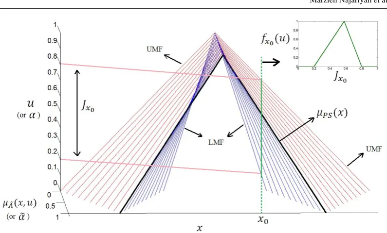
Definition 2 (Mendel 2008, Coupland and John 2007). A T2FS, ˜A, can be characterized by the so-called point-valued representation as follows:

˜

A={((x,u),µA˜(x,u))|∀x∈X,∀u∈Jx⊆[0,1]},

whereµA˜(x,u)anduare called type-2 membership

function and primary grade - or secondary variable - of ˜A, respectively,xis the primary variable,X is the domain of the fuzzy set, andJx is the domain

of the secondary membership function atx( see Fig. 1).

Definition 3 (Mendel and John 2002). Let ˜Abe a T2FS. A vertical slice of ˜Aatx0∈X,µA˜(x0), is a

T1FS and the membership function of secondary domain at the fixed pointx0. It is identified as:

µ_A˜(x0) =

∫

u∈Jx₀

fx0(u)/u

where fx0(u)is called secondary grade.

It should be noted that the integral sign stands for the union over all admissiblexand/oruis not stan-dard integration. Additionally, the sign′′/′′stands for association (or a marker) does not imply divi-sion.

Definition 4 (Mazandarani and Najariyan 2014a). An ˜α-cut set of the vertical slice of ˜Aat pointx0∈

X is defined as: S_A˜(x0|α˜) =

{

{u∈Jx0|fx0(u)≥α˜}, 0<α˜ ≤1,

cl{u∈Jx0|fx0(u)>α˜},α˜ =0,

wherecl(.)denotes the closure of the set, and it is compact.

Definition 5 (Liu 2008). Let ˜A be a T2FS. The union of all secondary domains of the T2FS whose secondary grades are greater or equal to ˜α∈[0,1]

is called ˜α-plane of ˜Aand denoted by ˜Aα˜ as:

˜ A_α˜ =

∫

x∈X

∫

u∈Jx

{(x,u)|S_A˜(x|α˜)}

˜ A_α˜ =

∫

x∈X

∫

u∈Jx

{(x,u)|fx(u)≥α˜}

Theorem 1 (Liu 2008).α˜-plane representation the-orem: A T2FS,A, can be represented as the union˜ of itsα˜-planes i.e.A˜=∪_α˜∈[0,1]α˜_A˜_α˜.

Definition 6 (Mazandarani and Najariyan 2014a, Hung and Yang 2004). Let ˜Aand ˜Bbe two type-2 fuzzy sets, anddH denote the well-known

Haus-dorff distance. A metric on the space of type-2 fuzzy sets is defined as follows:

d2(A,˜ B˜) =

∫ _b

a

Hf(µ_A˜(x),µB˜(x))dx

where

Hf(µA˜(x),µB˜(x)) =2

∫ 1

0

˜

αdH(SA˜(x|α˜),SB˜(x|α˜))dα˜

Definition 7 (Mazandarani and Najariyan 2014a,

Mendel et al. 2009). Suppose ˜A is a T2FS. The

˜

α-plane of the set at ˜α =0, ˜A0, is called

Fig. 1: A triangular type-2 fuzzy set with Lower Membership Function (LMF), Upper Membership Func-tion (UMF) and Principle Set (PS). Top insert depicts the secondary membership funcFunc-tion, i.e. vertical slice atx0

Note 1 The ˜α-plane of a T2FS, ˜A_α˜, is an

inter-val inter-valued fuzzy set, i.e. it is a set all of whose elements have interval membership grades (Ham-rawi 2011). That is, the T2FS at level ˜α , ˜A_α˜ , can

be characterized in a parametric form by the pair

(A_α˜,Aα˜)whereAα˜ is called Lower Membership

Function [LMF], andA_α˜ is called Upper

Mem-bership Function [UMF], and they are both T1FSs (Mazandarani and Najariyan 2014a).

Definition 8 (Hamrawi 2011). Let ˜Abe a T2FS. The ˜α-plane of the set at ˜α=1, ˜A1, is called

Prin-ciple Set [PS] of ˜A, and its membership function is defined as:

µPS(x) = ∫

x∈X

u/x s.t. fx(u) =1

Definition 9 (Hamrawi 2011,Hamrawi et al. 2010). Suppose ˜Ais a T2FS and its ˜α-plane is ˜Aα˜= (Aα˜,Aα˜).

Theα-cut of the ˜α-plane, ˜Aα_α˜, is theα-cut of its LMF and UMF, i.e. ˜Aα_α˜ = (A_αα_˜,Aα_α˜).

Theorem 2 (Hamrawi 2011,Hamrawi et al. 2010). A T2FS,A, can be represented by the union of all˜

itsα-cuts as follows:

˜ A= ∪

˜

α∈[0,1]

˜

α ∪

α∈[0,1] α_A˜α

˜

α

3 Triangular Perfect Quasi Type-2 Fuzzy Numbers

Definition 10 (Hamrawi 2011,Hamrawi et al. 2016, Mazandarani and Najariyan 2014b). A T2FS, ˜A, is called a perfect T2FN if the following conditions are satisfied:

1. UMF and LMF of FOU(A˜)are T1FNs them-selves,

2. UMF and LMF of PS of ˜A are T1FNs them-selves.

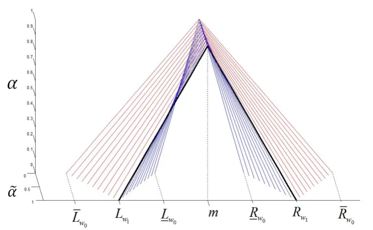
Fig. 2: A triangular perfect QT2FN, ˜w, withL_w

0,Rw0as the left and right endpoints of the support of LMF,

Lw0,Rw0as the left and right endpoints of the support of UMF,Lw1,Rw1as the left and right endpoints of

the support of PS andmas the core of the set

Note 2 (Hamrawi 2011). A perfect QT2FN can be completely determined using its FOU and PS.

A class of triangular perfect QT2FNs was intro-duced for the first time by Mazandarani and Na-jariyan in (Mazandarani and NaNa-jariyan 2014b) as the septuple

˜

w= (Lw0,Lw1,Lw0,m,Rw0,Rw1,Rw0) (1)

whereLw0≤Lw1≤Lw0 ≤m≤Rw0≤Rw1 ≤Rw0.

Fig. 2 shows the triangular perfect QT2FNs. The triangular perfect QT2FN, ˜w, in the levelsα and

˜

α, ˜wα_α˜ = (w_αα_˜,wα_α˜), is determined as:

            

wα_α˜ = [Lα_w

˜

α,R α

wα˜]

Lα_w

˜

α=Lαw1−(1−α˜)(L

α

w1−L

α

w0)

Rα_wα˜ =Rα_w

1−(1−α˜)(R

α

w1−R

α

w0)

(2) and

            

wα_α˜ = [Lα_w

˜

α,Rαwα˜]

Lα_w

˜

α =Lαw1−(1−α˜)(Lαw1−Lαw0)

Rα_w

˜

α=Rαw1−(1−α˜)(Rαw1−Rαw0)

(3)

whereLα_w

0 ≤L

α

w1 ≤L

α

w0 ≤R

α

w0 ≤R

α

w1≤R

α

w0, and

they are characterized as:

                                      

Lα_w

0 =m−(1−α)(m−Lw0)

Rα_w0=m−(1−α)(m−R_w0)

Lα_w

0 =m−(1−α)(m−Lw0)

Rα_w0=m−(1−α)(m−Rw0)

Lα_w1 =m−(1−α)(m−Lw1)

Rα_w

1=m−(1−α)(m−Rw1)

In the following some of the arithmetic operations on the triangular perfect QT2FNs are given. Let

˜

w= (Lw0,Lw1,Lw0,m,Rw0,Rw1,Rw0)and ˜z= (Lz0,

Lz1,Lz0,n,Rz0,Rz1,Rz0) be two triangular perfect

QT2FNs. The addition, ˜w+z, and scalar multipli-˜ cation byk∈R,kw, are defined as follows:˜

˜

w+z˜=(Lw0+Lz0,Lw1+Lz1,Lw0+Lz0,m+n,

R_w

0+Rz0,Rw1+Rz1,Rw0+Rw0)

kw˜= (kLw0,kLw1,kLw0,km,kRw0,kRw1,kRw0)

for k≥0,

kw˜= (kRw0,kRw1,kRw0,km,kLw0,kLw1,kLw0)

for k<0.

Moreover, the scalar multiplication byk∈R, ad-dition, subtraction, and multiplication, in the levels

αand ˜α are characterized as:

[kw˜]α_α˜ =

{

([kLα_wα˜,kRα_wα˜],[kLα_wα˜,kRα_wα˜]),k≥0,

([kRα_wα˜,kLα_wα˜],[kRα_wα˜,kLα_wα˜]),k<0.

and

[w˜◦z˜]α_α˜= ([wα_α˜◦zα_α˜],[wα_α˜◦zα_α˜])

where ˜w◦z˜means ˜w+z˜or ˜w−z˜or ˜w×z˜and

[wα_α˜◦zα_α˜] = [min{Lα_w

˜

α◦Lαzα˜,L

α

wα˜◦R

α

zα˜,R

α

wα˜◦L

α

zα˜,

Rα_w

˜

α◦Rαzα˜},

max{L_w

˜

α◦Lzα˜,Lwα˜◦Rzα˜,Rwα˜◦Lzα˜,

R_w

˜

α◦Rzα˜}]

[wα_α˜◦zα_α˜] = [min{Lα_w

˜

α◦L α

zα˜,L

α

wα˜◦R

α

zα˜,R

α

wα˜◦L

α

zα˜,

Rα_w

˜

α◦R α

zα˜},

max{Lwα˜ ◦Lzα˜,Lwα˜◦Rzα˜,Rwα˜◦Lzα˜,

Rwα˜ ◦Rzα˜}]

4 Type-2 Fuzzy Linear System

This section presents a class of T2FLS in which the coefficients are real crisp numbers and the vari-ables are the triangular perfect QT2FNs. An ap-proach, similar to what was proposed in (Fried-man et al. 1998), is introduced for obtaining the solution of T2FLS. In order for ideas to flow bet-ter and easier to follow the notations used in this section are tried to be compatible with that used in (Friedman et al. 1998). Moreover, a definition of the type-2 fuzzy solution is presented.

A system of linear equations as:

        

a11x˜1+a12x˜2+···+a1nx˜n=y˜1

a21x˜1+a22x˜2+···+a2nx˜n=y˜2

.. .

an1x˜1+an2x˜2+···+annx˜n=y˜n

(5)

whereai j∈R,1≤i,j≤nand ˜xi,y˜i∈E2is called

a T2FLS. T2FLS shown in Eq. (5) is expressed in the matrix form asAX˜ =_Y˜ _{in which}

A= [ai j]n×n, X˜= [x˜1x˜2···x˜n]T

and

˜

Y = [y˜1y˜2 ···y˜n]T

According to Definition9, we have

(xα_iα˜,xα_iα˜) = ([Lα_x

iα˜,Rαxiα˜],[L

α

xiα˜,R

α

xiα˜])

and

(yα

iα˜,y

α

i_α˜) = ([Lαyiα˜,Rαyiα˜],[L

α

yiα˜,R

α

yiα˜])

Based on Theorem2, solving T2FLS shown in Eq. (5) is equivalent to obtaining a solution of the fol-lowing equations system:

                    

Lα[ ∑n

j=1ai jx˜j

] ˜

α

=∑n_j=1Lα[

ai jx˜j

] ˜

α

=Lα_y iα˜

Rα[ ∑n

j=1ai jx˜j

] ˜

α

=∑n_j=1Rα[

ai jx˜j

] ˜

α

=Rα_y iα˜

Lα[ ∑n

j=1ai jx˜j

] ˜

α

=∑n_j=1Lα[

ai jx˜j

] ˜

α

=Lα_y iα˜

Rα[ ∑n

j=1ai jx˜j

] ˜

α

=∑n_j=1Rα[

ai jx˜j

] ˜

α

=Rα_y iα˜

The system given by equations shown in Eq. (6) is a 4n×4ncrisp linear system where the right-hand side column is the 4n×1 matrix

[

Lα_{y1 ˜}

α ··· Lαynα˜ Ry1 ˜α_α ···Rαynα˜ L

α

y1 ˜_α ···L

α

ynα˜ R

α

y1 ˜_α

···Rα_y nα˜

]T

.

System shown in Eq. (6) can be rewritten in order that the 4n×1 matrix

X_α,_α˜ = [

Lα_x

1 ˜α ···L

α

xnα˜ −R

α

x1 ˜α ··· −R

α

xnα˜ L

α

x1 ˜α

···Lα_x nα˜ −R

α

x1 ˜α ··· −R

α

xnα˜ ]T

includes the unknown variables, and the 4n×1 matrix including the known variables in the right-hand side is

Y_α,α˜ = [

Lα_{y1 ˜}

α ···Lαynα˜ −Rαy1 ˜_α ··· −Rαynα˜

Lα_y

1 ˜α ···L α

ynα˜ −R

α

y1 ˜α ··· −R α

ynα˜ ]T

. (7)

This rearranging leads to the systemSX_α,_α˜ =Y_α,_α˜

whereSis a real 4n×4nsquare matrix in the form of S=    

B C0 0 C B0 0 0 0 B C 0 0 C B

  

 (8)

in which 0 denotes ann×nzero matrix and the matricesB= [bi j]n×n,C= [ci j]n×n, are

nonnega-tive matrices whose entries are determined as: bi j=

{

ai jai j>0

0 ai j≤0

ci j= {

−ai jai j<0

0 ai j≥0

(9)

It is easy to see thatA=B−C. It should be noted, if system shown in Eq. (6) does not have a unique solution, then T2FLS shown in Eq. (5) does not have a unique solution either. The unique solution to system shown in Eq. (6) can be found if and only if the matrixSis invertible.

Theorem 3 The matrix S is invertible if and only if the matrices A and B+C are both invertible.

Proof It is similar to the proof of Theorem 1 in (Friedman et al. 1998).

Based on Theorem 3 presented in (Friedman et al. 1998), a special case of T1FLSs has a unique fuzzy solution. What follows is a corollary of the Theo-rem 3 in the context of T2FLSs.

Corollary 1 T2FLS shown in Eq. (5) has a type-2 fuzzy solution, belonging to the triangular perfect QT2FNs, providing that matrix S has an inverse matrix, S−1_{, whose entries are nonnegative.}

Proof For the proof of this theorem what is needed is to prove that Lα_x

iα˜ ≤L

α

xiα˜ ≤R

α

xiα˜ ≤R

α

xiα˜. It is

straightforward and hence omitted.

Although the conditions in Corollary 1 are suf-ficient conditions, and assure us that the unique type-2 fuzzy solution can be obtained, there is scarcely any matrix S which satisfies the conditions. As a result, the following definition of solution is given.

Definition 12 SupposeS−1is the inverse of ma-trixS, andZ_α,_α˜ = [zl(α,α˜)]4n×1,l=1,2, ...,4n, is

a solution of SZ_α,α˜ =Yα,α˜, i.e.Zα,α˜ =S−1Yα,α˜.

We say that ˜X= [x˜1x˜2 ···x˜n]T is the type-2 fuzzy

solution of T2FLS shown in Eq. (5) provided that ˜

xi=

∪

˜

α∈[0,1]

˜

α ∪

α∈[0,1]

αx˜α_iα˜ ∀i=1,2, ...,n

represents the triangular perfect QT2FN where ˜

x_iα_α˜ = (xα_iα˜,xα_iα˜) = ([Lα_x

iα˜,Rαxiα˜],[L

α

xiα˜,R

α

xiα˜]),

and       

Lα_x

iα˜ =zi(α,α˜)

−Rα_x

iα˜ =zi+n(α,α˜)

Lα_x

iα˜ =zi+2n(α,α˜)

−Rα_x

iα˜ =zi+3n(α,α˜)

(10)

Based on the aforementioned, the following steps can be cosidered for obtaining the unique fuzzy solution of T2FLS shown in Eq. (5):

Step 1.Set up the matricesY_α,α˜ andSaccording

to the relations shown in Eqs. (7), (8), and (9) re-spectively.

i.e. |S| ̸=0, then S−1 _{exists, and go to the next}

step. If the determinant of the matrixSis zero, i.e. |S|=0, thenS−1does not exist, and therefore the problem does not have a unique fuzzy solution. Step 3.ObtainZ_α,α˜= [zl(α,α˜)]4n×1,l=1,2, ...,4n

usingZ_α,α˜ =S−1Yα,α˜.

Step 4.Using Eq. (10), determineLα_x

iα˜,Rαxiα˜,L

α

xiα˜,

andRα_x

iα˜ for each ˜xαi_α˜.

Step 5.Check whether([Lα_x

iα˜,Rαxiα˜],[L

α

xiα˜,R

α

xiα˜]),i=

1,2, ...,nrepresents a T2FN or not. To do that, we need to check whether the LMF, i.e. [Lα_x

iα˜,Rαxiα˜]

and UMF, i.e.[Lα_x iα˜,R

α

xiα˜] are T1FNs them selves

or not. If the LMF and UMF are T1FNs for each i=1,2, ...,n, andLα_w

˜

α ≤Lαwα˜ ≤Rαwα˜ ≤R

α

wα˜ then

according to Definition10 ˜

xα_iα˜= (xα_iα˜,xα_iα˜) = ([Lα_x

iα˜,Rαxiα˜],[L

α

xiα˜,R

α

xiα˜])

represents a T2FN. Moreover, based on Definition 12x˜α_iα˜ = (x_iα_α˜,xα_iα˜)is the unique fuzzy solution of T2FLS shown in Eq. (5) which can be character-ized in the form of the septuple shown in Eq. (1). Step 6.The unique fuzzy solution of T2FLS shown in Eq. (5) can be represented in the septuple form shown in Eq. (1) as

˜ xi=

(

Lxi0,Lxi1,Lxi0,m,Rxi0,Rxi1,Rxi0 )

where, based on the relations shown in Eqs. (2), (3), and (4) ,

Lxi0 =L

α

xiα˜α˜,α=0, Lxi1=L

α

xiα˜α˜=1,α=0,

L_x i0 =L

α

xiα˜α˜,α=0, m=Lαxiα˜α˜,α=1,

Rxi0 =R

α

xiα˜α˜,α=0, Rxi1 =R

α

xiα˜α˜=1,α=0,

R_x i0 =R

α

xiα˜α˜,α=0.

5 Examples

Example 1 A stage in the retrofit strategy for the reduction of water and energy in pulp and paper processes is considered as an application of type-2 fuzzy linear system. The stage corresponds to pulp washing process. Pulp and paper are manu-factured from raw materials containing cellulose

fibers, generally wood, recycled paper, and agri-cultural residues (Bajpai 2012). The process of pulp washing has been shown in Fig. 3 which has been adopted from (Patino and Nunez 1998).

In this case, we are going to obtain the values of the pulp flowing out from filter 1, 2 and the wastew-ater from filter 2. The unknowns are concentra-tions. The information has been obtained by the aim of the experiences of an expert and others with a level lower than that of the expert. Depending on their experience and expertise, the experts men-tion different uncertainty for the concentramen-tion val-ues of pulp flowing into the blow tank, wastewater flowing out filter 1 and pulp flowing into filter 3. If it is not possible to present an exact form of a type-1 fuzzy number for each of the values, in which the specialized experience ofallthe experts with different levels of expertise are reflected hierarchi-cally, then type-2 fuzzy numbers may prove help-ful in this case. This could be considered in the way that the more reliable an expert’s experience, compared to all of the others’, the higher ˜α-plane includes his/her membership functions. Using the mass balance for each species the following equa-tions are obtained



280 30 500 30 50 280 0 50

   cc˜˜68

˜ c9

 =

 83 ˜65 ˜cc15

785 ˜c12   (11) where    ˜

c1= (5,7,8,10,12,13,15),

˜

c5= (1.5,1.7,1.8,2,2.2,2.3,2.5),

˜

c12= (0.5,0.7,0.8,1,1.2,1.3,1.5).

(12)

According to the steps expressed in the previous section we have:

Step 1.According to the relation shown in Eq. (7) we have:

Y_α,_α˜ = [

83Lα_c

1 ˜α 65L

α

c5 ˜α785Lαc12 ˜α −83R

α

c1 ˜α −65R

α

c5 ˜α −785Rα_c

12 ˜α83L α

c1 ˜α65L α

c5 ˜α 785L α

c12 ˜α −83R α

c1 ˜α −65Rα_c

5 ˜α −785R

α

Fig. 3: The process of pulp washing. Originally published in (Patino and Nunez 1998) under CC BY-NC-SA 3.0 license. Available from: http://dx.doi.org/10.5772/20882.

where, based on the relations shown in Eqs. (2), (3), and (4),

Lα_c

1 ˜α=7+3α−(1−α˜)(α−1)

Rα_{c1 ˜}

α=13−3α−(1−α˜)(1−α) Lα_c

1 ˜α=7+3α−(1−α˜)(2−2α)

Rα_c

1 ˜α=13−3α−(1−α˜)(2α−2)

Lα_{c5 ˜}

α=1.7+0.3α−(1−α˜)(0.1α−0.1) Rα_c

5 ˜α=2.3−0.3α−(1−α˜)(0.1−0.1α)

Lα_c

5 ˜α=1.7+0.3α−(1−α˜)(0.2−0.2α)

Rα_c

5 ˜α=2.3−0.3α−(1−α˜)(0.2α−0.2)

Lα_c

12 ˜α=0.7+0.3α−(1−α˜)(0.1α−0.1)

Rα_c

12 ˜α =1.3−0.3α−(1−α˜)(0.1−0.1α)

Lα_c

12 ˜α=0.7+0.3α−(1−α˜)(0.2−0.2α)

Rα_c

12 ˜α =1.3−0.3α−(1−α˜)(0.2α−0.2)

and by the use of the relations shown in Eqs. (8) and (9) we have

S=

   

B0 0 0 0 B0 0 0 0 B0 0 0 0 B

   

in which

B=



280 30 500 30 50 280 0 50

 

Step 2.The determinant of the matrix Sis |S|=

|B|4̸=0, thenSis invertible and we go to the next step.

Step 3. The matrix Z_α,α˜ = [zl(α,α˜)]12×1 is

ob-tained as:

z1(α,α˜) =1.68+0.82α−(1−α˜)(0.27α−0.27)

z2(α,α˜) =1.05+0.45α−(1−α˜)(0.15α−0.15)

z3(α,α˜) =1.58+0.12α−(1−α˜)(0.04α−0.04)

z4(α,α˜) =−3.32+0.82α−(1−α˜)(0.27α−0.27)

z5(α,α˜) =−1.95+0.45α−(1−α˜)(0.15α−0.15)

z6(α,α˜) =−1.82+0.12α−(1−α˜)(0.04α−0.04)

z7(α,α˜) =1.68+0.82α−(1−α˜)(0.55−0.55α)

z8(α,α˜) =1.05+0.45α−(1−α˜)(0.3−0.3α)

z9(α,α˜) =1.58+0.12α−(1−α˜)(0.08−0.08α)

z10(α,α˜) =−3.32+0.82α−(1−α˜)(0.55−0.55α)

z11(α,α˜) =−1.95+0.45α−(1−α˜)(0.3−0.3α)

Step 4.Using the relation shown in Eq. (10) we have:

Lα_c

6 ˜α=1.68+0.82α−(1−α˜)(0.27α−0.27)

Rα_c

6 ˜α =3.32−0.82α+ (1−α˜)(0.27α−0.27)

Lα_c

6 ˜α=1.68+0.82α−(1−α˜)(0.55−0.55α)

Rα_c

6 ˜α =3.32−0.82α+ (1−α˜)(0.55−0.55α)

Lα_{c8 ˜}

α=1.05+0.45α−(1−α˜)(0.15α−0.15) Rα_{c8 ˜}

α =1.95−0.45α+ (1−α˜)(0.15α−0.15) Lα_{c8 ˜}

α=1.05+0.45α−(1−α˜)(0.3−0.3α) Rα_{c8 ˜}

α =1.95−0.45α+ (1−α˜)(0.3−0.3α) Lα_{c9 ˜}

α=1.58+0.12α−(1−α˜)(0.04α−0.04) Rα_c

9 ˜α =1.82−0.12α+ (1−α˜)(0.04α−0.04)

Lα_c

9 ˜α=1.58+0.12α−(1−α˜)(0.08−0.08α)

Rα_c

9 ˜α =1.82−0.12α+ (1−α˜)(0.08−0.08α)

Step 5.It is easy to see that[Lα_c

6 ˜α,R

α

c6 ˜α]represents

theα-level sets of a T1FN for each ˜α∈[0,1], and

[Lα_c

6 ˜α,R

α

c6 ˜α] does too. Additionally, since L

α

c6 ˜α ≤

Lα_{c6 ˜}

α ≤Rαc6 ˜_α≤R

α

c6 ˜_α, then

[c˜6]αα˜ = ([Lαc6 ˜α,R

α

c6 ˜α],[L

α

c6 ˜α,R

α

c6 ˜α])

represents a T2FN. In a similar way, it can be in-vestigated that[c˜8]αα˜= ([Lcα8 ˜α,Rαc8 ˜α],[L

α

c8 ˜α,R α

c8 ˜α])and

[c˜9]α_α˜= ([Lαc9 ˜α,R

α

c9 ˜α],[L

α

c9 ˜α,R

α

c9 ˜α])also represent two

T2FNs.

Step 6. Consequently, the fuzzy solution of the system shown in Eq. (11) can be characterized in the septuple form as:

  

˜

c6= (1.13,1.68,1.95,2.5,3.05,3.32,3.87),

˜

c8= (0.75,1.05,1.2,1.5,1.8,1.95,2.25),

˜

c9= (1.5,1.58,1.62,1.7,1.78,1.82,1.9).

As a result, based on the multiplication of a scalar by a T2FN defined in section 3, the values of the pulp flowing out from filter 1, 2 and the wastewater from filter 2 are obtained by the multiplication of

f6by ˜c6, f8by ˜c8andf9by ˜c9, respectively, as

f6c˜6= (316.4,470.4,546,700,854,929.6,1083.6),

f8c˜8= (22.5,31.5,36,45,54,58.5,67.5),

and

f9c˜9= (75,79,81,85,89,91,95)

which mean approximately 700, 45, and 85. It should be noted that using the obtained results, approxi-mately 700 also means the T1FN(470.4,700,929.6)

whose uncertainty dispersion can be considered by its UMF and LMF as(316.4,700,1083.6)and(546, 700,854), respectively. The uncertainty dispersion for approximately 45 and 85 can also be expressed in a similar way. Needless to pinpoint once more that, unlike T2FLSs, T1FLSs cannot provide any information about the uncertainty dispersion of the results.

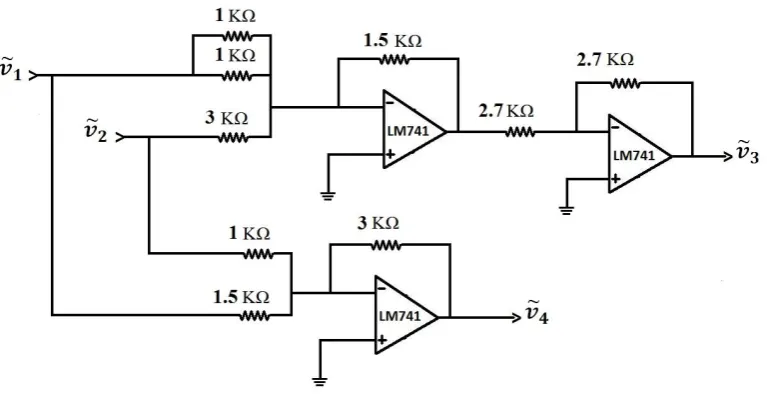
Example 2 Consider the electrical circuit shown in Fig. 4 where ˜v1, ˜v2are the input voltages, and

˜

v3, ˜v4are the output voltages. The circuit is a kind

of summing amplifier with two inputs and two out-puts. The relationship between input and output voltages is as follows:

[

3 0.5 −2−3

][

˜ v1

˜ v2

]

=

[

˜ v3

˜ v4

]

(13)

What we are investigating is determining the in-put voltages on condition that the outin-put voltages are known but uncertain. That is, e.g. ˜v3is ”about

16(volt)”, and ˜v4is ”about−16(volt)”. Assume,

the engineers’ expert ideas about the uncertainty of output voltages differ. If we prefer to consider the interpretation of just one, not all of the experts, the linear system shown in Eq. (13) will be a T1FLS one, failing to consider the interpretation or expe-rience of the other experts. Alternatively, we may consider a form of T1FN for each of the output voltages, based on the experiences of the experts that, in turn, leads to the presentation of T1FLS. Even this model of system fails to hierarchically reflect the specialized experience ofallthe experts with different levels of expertise. However, each of the output voltages may be determined using a triangular perfect QT2FN as shown in figures 5 and 6. For determining the input voltages, the ma-trixZ_α,α˜ = [zl(α,α˜)]8×1is needed to be obtained.

Then, according to the steps expressed in the pre-vious section we have:

Step 1.The matricesSandY_α,_α˜ can be gained

Fig. 4: The electrical circuit considered in Example 2

(7), respectively, as follows:

S=

           

3 0.5 0 0 0 0 0 0 0 0 −2−3 0 0 0 0 0 0 3 0.5 0 0 0 0 −2−3 0 0 0 0 0 0 0 0 0 0 3 0.5 0 0 0 0 0 0 0 0 −2−3 0 0 0 0 0 0 3 0.5 0 0 0 0 −2−3 0 0

           

Y_α,α˜ = [

Lα_{v3 ˜}

α Lαv4 ˜_α −Rαv3 ˜_α −Rαv4 ˜_αL

α

v3 ˜_α

Lα_v

4 ˜α −R

α

v3 ˜α −R

α

v4 ˜α ]T

where, based on the relations shown in Eqs. (2), (3), and (4),

Lα_v

3 ˜α=14+2α−(1−α˜)(α−1),L

α

v4 ˜α=−R

α

v3 ˜α

Rα_v

3 ˜α=18−2α−(1−α˜)(1−α),R

α

v4 ˜α=−L

α

v3 ˜α

Lα_v

3 ˜α=14+2α−(1−α˜)(1−α),L

α

v4 ˜α=−R

α

v3 ˜α

Rα_v

3 ˜α=18−2α−(1−α˜)(α−1),R

α

v4 ˜α=−L

α

v3 ˜α

Step 2.The determinant of the matrixS is|S|=

4096, then the matrixSis invertible and we go to the next step.

Step 3.The matrixZ_α,α˜ = [zl(α,α˜)]8×1is

deter-mined as:

z1(α,α˜) =4.37+0.63α−(1−α˜)(0.32α−0.32)

z2(α,α˜) =1.75+0.25α−(1−α˜)(0.13α−0.13)

z3(α,α˜) =−5.63+0.63α−(1−α˜)(0.32α−0.32)

z4(α,α˜) =−2.25+0.25α−(1−α˜)(0.13α−0.13)

z5(α,α˜) =4.37+0.63α−(1−α˜)(0.31−0.31α)

z6(α,α˜) =1.75+0.25α−(1−α˜)(0.12−0.12α)

z7(α,α˜) =−5.63+0.63α−(1−α˜)(0.31−0.31α)

z8(α,α˜) =−2.25+0.25α−(1−α˜)(0.12−0.12α)

Step 4.Using the relation shown in Eq. (10) we have:

Lα_{v1 ˜}

α =4.37+0.63α−(1−α˜)(0.32α−0.32), Rα_v

1 ˜α=5.63−0.63α+ (1−α˜)(0.32α−0.32),

Lα_v

1 ˜α =4.37+0.63α−(1−α˜)(0.31−0.31α),

Rα_v

1 ˜α=5.63−0.63α+ (1−α˜)(0.31−0.31α),

Lα_v

2 ˜α =1.75+0.25α−(1−α˜)(0.13α−0.13)

Rα_v

2 ˜α=2.25−0.25α+ (1−α˜)(0.13α−0.13)

Lα_v

2 ˜α =1.75+0.25α−(1−α˜)(0.12−0.12α)

Rα_v

2 ˜α=2.25−0.25α+ (1−α˜)(0.12−0.12α)

Step 5.It is easy to see that[Lα_v

1 ˜α,R

α

v1 ˜α]represents

theα-level sets of a T1FN for each ˜α∈[0,1], and

[Lα_{v1 ˜} α,R

α

v1 ˜_α] does too. Additionally, since L

α

Lα_{v1 ˜}

α ≤Rαv1 ˜_α≤R

α

v1 ˜_α, then

[v˜1]αα˜ = ([Lαv1 ˜α,R

α

v1 ˜α],[L

α

v1 ˜α,R

α

v1 ˜α])

represents a T2FN. In a similar way, it can be in-vestigated that[v˜2]αα˜= ([Lαv2 ˜α,R

α

v2 ˜α],[L

α

v2 ˜α,R

α

v2 ˜α])also

represents a T2FN.

Step 6.Eventually, the input voltages can be ex-pressed as:

˜

v1= (4.06,4.37,4.69,5,5.31,5.63,5.94),

˜

v2= (1.63,1.75,1.88,2,2.12,2.25,2.37),

The input voltages ˜v1and ˜v2are two T2FNs whose

cores are 5 and 2, respectively. Due to uncertainty, they are not exactly 5 and 2, but they can be in-terpreted as approximately 5 and approximately 2. As a result, one can interpret that the circuit ampli-fies approximately 5 and 2 (volt) to approximately 16 and−16 (volt), respectively.

6 Conclusion

In this paper, a model of fuzzy linear system called T2FLS has been established that enables us to model linear systems in which in addition to data, the membership function itself is uncertain. T2FLS, unlike T1FLS, provides information about uncer-tainty dispersion. It was shown that how ann×n T2FLS is replaced by a 4n×4ncrisp linear system. Furthermore, the conditions for the existence of a unique type-2 fuzzy solution to then×nT2FLS was given. Since the conditions may not always occur, a definition of type-2 fuzzy solution has been defined. Using two examples in the pulp and pa-per industry and electrical engineering we showed that how the T2FLSs enable the decision maker to model the system with different interpretations of uncertainty expressed by experts in different lev-els. Due to the fact that T2FLSs with the help of T2FNs model higher levels uncertainty than those do the T1FLSs, this opens up an efficient way for modeling linear system and human decision mak-ing. We believe that what have been presented in this paper can be used to extend many existing T1FLSs result to T2FLSs. The next step in the

research direction proposed here is to investigate T2FLSs in which all the variables and coefficients are T2FNs.

References

Abbasbandy S, Ezzati R, Jafarian A (2006) LU de-composition method for solving fuzzy system of linear equations. Appl. Math. Comput. 172:633-643

Abbasbandy S, Jafarian A (2006) Steepest descent method for system of fuzzy linear equations. Ap-plied Mathematics and Computation 175:823-833 Bajpai P (2012) Biotechnology for Pulp and Paper Processing. Springer US

Behera D, Chakraverty S (2014) Solving fuzzy complex system of linear equations. Information Sciences 277:154-162

Buckley JJ, Qu Y (1991) Solving systems of linear fuzzy equations. Fuzzy Sets and Systems 43:33-43 Coupland S, John RI (2007) Geometric Type-1 and Type-2 Fuzzy Logic Systems. IEEE Transactions on Fuzzy Systems 15:3-15

Das S, Kar S, Pal T (2017) Robust decision mak-ing usmak-ing intuitionistic fuzzy numbers. Granul Comput doi:10.1007/s41066-016-0024-3

Friedman M, Ming M, Kandel A (1998) Fuzzy lin-ear systems. Fuzzy Sets and Systems 96:201-209 Ghanbari R (2015) Solutions of fuzzy LR alge-braic linear systemsusing linear programs. Ap-plied Mathematical Modelling 39:5164-5173 Garibaldi JM, Zhou SM, Wang XY, John RI, El-lis IO (2012) Incorporation of Expert Variability into Breast Cancer Treatment Recommendation in Designing Clinical Protocol Guided Fuzzy Rule System Models. Journal of Biomedical Informat-ics 45:447-459

Fig. 5: The output voltage, ˜v3, corresponding to the electrical circuit

Fig. 6: The output voltage, ˜v4, corresponding to the electrical circuit

fuzzy sets. In: IEEE international confer-ence on fuzzy systems, Barcelona, Spain, doi:10.1109/FUZZY.2010.5584783

Hamrawi H (2011) Type-2 fuzzy alpha-cuts. Ph.D. Dissertation, De Montfort University.

Hamrawi H, Coupland S, John RI (2016) Type-2 fuzzy alpha-cuts. IEEE Transactions on Fuzzy Systems, doi:10.1109/TFUZZ.2016.2574914

Hung WL, Yang MS (2004) Similarity measures between type-2 fuzzy sets. Int J Uncertainty Fuzzi-ness Knowledge-Based Syst 12:827-41

Liu F (2008) An efficient centroid type-reduction strategy for general type-2 fuzzy logic system, In-formation Sciences 178:2224-2236

Mendel JM (2007) Type-2 fuzzy sets and systems: an overview. IEEE Comput Intell Mag 2:20-9 Mendel JM, Liu F (2008) On new quasi-type-2 fuzzy logic systems. In: Proceeding of 2008 in-ternational conference on fuzzy systems, Proceed-ings of the 2008 IEEE International Conference on Fuzzy Systems, Hong Kong, China, pp. 354-360 Mendel JM (2016) A comparison of three ap-proaches for estimating (synthesizing) an interval type-2 fuzzy set model of a linguistic term for computing with words. Granul Comput 1:59-69 Ming M, Friedman M, Kandel A (2000) Duality in fuzzy linear systems. Fuzzy Sets and Systems 109:55-58

Mendel JM, John RI (2002) Type-2 fuzzy sets made simple. IEEE Transactions on Fuzzy Sys-tems 10:117-127

Mazandarani M, Kamyad AV (2011) A practi-cal approach to prescribe the amount of used in-sulin of diabetic patients. 19th Iranian Conference on Electrical Engineering, Tehran, Iran, pp. 3158-3162

Mendel JM, Liu F, Zhai D (2009)α-Plane repre-sentation for type-2 fuzzy sets: theory and applica-tions. IEEE Trans Fuzzy Syst 17:1189-207 Mazandarani M, Najariyan M (2014) Type-2 fuzzy fractional derivatives. Commun Nonlinear Sci Nu-mer Simulat 19:2354-2372

Mazandarani M, Najariyan M (2014) Differentia-bility of type-2 fuzzy number-valued Functions. Commun Nonlinear Sci Numer Simul 19:710-25 Muzzioli S, Reynaerts H (2006) fuzzy linear sys-tems of the formA1x+b1=A2X+b2. Fuzzy Sets

and Systems 157:939-951

Najariyan M, Farahi MH, Alavian M (2011) Op-timal control of HIV infection by using fuzzy dy-namical systems. J Math Comput Sci 2: 639-49

Najariyan M, Farahi MH (2015) A new approach for solving a class of fuzzy optimal control sys-tems under generalized Hukuhara differentiability. Journal of the Franklin Institute 352:1836-1849 Najariyan M, Mazandarani M (2015) A note on ”Numerical solutions for linear system of first-order fuzzy differential equations with fuzzy con-stant coefficients”. Information Sciences 305:93-96

Patino M, Nunez MP (2011) Retrofit Approach forthe Reduction of Water and Energy Consump-tion in Pulp and Paper ProducConsump-tion Processes. En-vironmental Management in Practice, Dr. Elzbi-etaBroniewicz (Ed.) doi: 10.5772/20882

Tian Z, Hu L, Greenhalgh D (2010) Perturbation analysis of fuzzy linear systems. Information Sci-ences 180:4706-4713

Wang C, Xinggan Fu, Meng S, He Y (2017) SPIF-GIA operators and their applications to decision making. Granul Comput doi:10.1007/s41066-016-0025-2

Wang X, Zhong Z, Ha M (2001) Iteration algo-rithms for solving a system of fuzzy linear equa-tions. Fuzzy Sets and Systems 119:121-128 Zadeh LA (1975) The concept of a linguistic vari-able and its application to approximate reasoning-1. Inf Sci 8:199-249.