A continuous time formulation for spatial capture recapture models

Full text

(1)A CONTINUOUS-TIME FORMULATION FOR SPATIAL CAPTURE-RECAPTURE MODELS Greg Distiller A Thesis Submitted for the Degree of PhD at the University of St Andrews. 2017 Full metadata for this item is available in St Andrews Research Repository at: http://research-repository.st-andrews.ac.uk/. Please use this identifier to cite or link to this item: http://hdl.handle.net/10023/15596. This item is protected by original copyright.

(2) A Continuous-Time Formulation for Spatial Capture-Recapture Models Greg Distiller A thesis presented for the degree of Doctor of Philosophy. 1. Department of Statistical Sciences Statistics in Ecology, Environment and Conservation (SEEC) University of Cape Town, South Africa 2. School of Mathematics and Statistics Centre for Research into Ecological and Environmental Modelling (CREEM) University of St Andrews, United Kingdom December 2, 2016.

(3)

(4) A Continuous-Time Formulation for Spatial Capture-Recapture Models Greg Distiller Abstract Spatial capture-recapture (SCR) models are relatively new but have become the standard approach used to estimate animal density from capture-recapture data. It has in the past been impractical to obtain sufficient data for analysis on species that are very difficult to capture such as elusive carnivores that occur at low density and range very widely. Advances in technology have led to alternative ways to virtually “capture” individuals without having to physically hold them. Some examples of these new non-invasive sampling methods include scat or hair collection for genetic analysis, acoustic detection and camera trapping. In traditional capture-recapture (CR) and SCR studies populations are sampled at discrete points in time leading to clear and well defined occasions whereas the new detector types mentioned above sample populations continuously in time. Researchers with data collected continuously currently need to define an appropriate occasion and aggregate their data accordingly thereby imposing an artificial construct on their data for analytical convenience. This research develops a continuous-time (CT) framework for SCR models by treating detections as a temporal non homogeneous Poisson process (NHPP) and replacing the usual SCR detection function with a continuous detection hazard function. The general CT likelihood is first developed for data from passive (also called “proximity”) detectors like camera traps that do not physically hold individuals. The likelihood is then modified to produce a likelihood for single-catch traps (traps that are taken out of action by capturing an animal) that has proven difficult to develop with a discrete-occasion approach. The lack of a suitable single-catch trap likelihood has led to researchers using a discrete-time (DT) multi-catch trap estimator to analyse single-catch trap data. Previous work has found the DT multi-catch estimator to be robust despite the fact that it is known to be based on the wrong model for single-catch traps (it assumes that the traps continue operating after catching an individual). Simulation studies in this work confirm that the multi-catch estimator is robust for estimating density when density is constant or does not vary much in space. However, there are scenarios with ii.

(5) non-constant density surfaces when the multi-catch estimator is not able to correctly identify regions of high density. Furthermore, the multi-catch estimator is known to be negatively biased for the intercept parameter of SCR detection functions and there may be interest in the detection function in its own right. On the other hand the CT single-catch estimator is unbiased or nearly so for all parameters of interest including those in the detection function and those in the model for density. When one assumes that the detection hazard is constant through time there is no impact of ignoring capture times and using only the detection frequencies. This is of course a special case and in reality detection hazards will tend to vary in time. However when one assumes that the effects of time and distance in the time-varying hazard are independent, then similarly there is no information in the capture times about density and detection function parameters. The work here uses a detection hazard that assumes independence between time and distance. Different forms for the detection hazard are explored with the most flexible choice being that of a cyclic regression spline. Extensive simulation studies suggest as expected that a DT proximity estimator is unbiased for the estimation of density even when the detection hazard varies though time. However there are indirect benefits of incorporating capture times because doing so will lead to a better fitting detection component of the model, and this can prevent unexplained variation being erroneously attributed to the wrong covariate. The analysis of two real datasets supports this assertion because the models with the best fitting detection hazard have different effects to the other models. In addition, modelling the detection process in continuous-time leads to a more parsimonious approach compared to using DT models when the detection hazard varies in time. The underlying process is occurring in continuous-time and so using CT models allows inferences to be drawn about the underlying process, for example the timevarying detection hazard can be viewed as a proxy for animal activity. The CT formulation is able to model the underlying detection hazard accurately and provides a formal modelling framework to explore different hypotheses about activity patterns. There is scope to integrate the CT models developed here with models for space usage and landscape connectivity to explore these processes on a finer temporal scale. SCR models are experiencing a rapid growth in both application and method development. The data generating process occurs in CT and hence a CT modelling approach is a natural fit and opens up several opportunities that are not possible with a DT formulation. The work here makes a contribution by developing and exploring the utility of such a CT SCR formulation.. iii.

(6) Publications resulting from this PhD dissertation • Distiller, G. and Borchers, D. (2015) A spatially explicit capture-recapture estimator for single-catch traps. Ecology and Evolution 5 (21): 5075-5087. • Borchers, D., Distiller, G., Foster, R., Harmsen, B., and Milazzo, L. (2014) Continuous-time spatially explicit capture-recapture models, with an application to a jaguar camera-trap survey. Methods in Ecology and Evolution 5 (7): 656665. doi: 10.1111/2041-210X.12196. iv.

(7) Acknowledgements I have learnt a great deal over the course of this research and my heartfelt thanks go out to my primary supervisor Prof David Borchers for all his input and wisdom. Without him this project would never have been conceived and made a reality. I would also like to thank my local supervisor Dr Birgit Erni for always being prepared to listen to my obscure questions and for providing assistance wherever she could. Thanks are due to Rebecca Foster and Bart Harmsen for making the jaguar camera-trap data available for this study. Collection of camera-trap data was funded by Panthera, with field and logistical assistance provided by the University of Belize’s Environmental Research Institute and the Belize Audubon Society. Thanks also to Phil Cowan and Landcare Research Manaaki Whenua, New Zealand for making the possum timing data available. I also thank the Engineering and Physical Sciences Research Council (EPSRC) for funding this work (EPSRC grant EP/I000917/1). Last but not least I acknowledge my wife Suki for all the support she has given me and for putting up with me during the difficult moments, and to my beautiful children Amy and Ruben who bring so much light into my life.. v.

(8) vi.

(9) Contents 1 Introduction 1.1 Estimating animal density . . . . . . . . . 1.2 Capturing in continuous-time . . . . . . . 1.3 Continuous-time models . . . . . . . . . . 1.4 Single-catch traps . . . . . . . . . . . . . . 1.5 Applications . . . . . . . . . . . . . . . . . 1.5.1 Jaguars in Belize . . . . . . . . . . 1.5.2 Brushtail possums in New Zealand 1.6 Objective and overview . . . . . . . . . . .. . . . . . . . .. . . . . . . . .. . . . . . . . .. . . . . . . . .. . . . . . . . .. . . . . . . . .. . . . . . . . .. . . . . . . . .. . . . . . . . .. . . . . . . . .. . . . . . . . .. . . . . . . . .. . . . . . . . .. . . . . . . . .. . . . . . . . .. 1 1 3 5 6 7 7 8 9. 2 A continuous-time spatial capture-recapture formulation 13 2.1 Spatial capture recapture: discrete-time formulation . . . . . . . . . . 13 2.1.1 Notation . . . . . . . . . . . . . . . . . . . . . . . . . . . . . . 14 2.1.2 General likelihood . . . . . . . . . . . . . . . . . . . . . . . . . 15 2.1.3 The spatial detection function . . . . . . . . . . . . . . . . . . 17 2.1.4 Detector types . . . . . . . . . . . . . . . . . . . . . . . . . . 19 2.2 Spatial capture recapture: continuous-time formulation for proximity detectors . . . . . . . . . . . . . . . . . . . . . . . . . . . . . . . . . . 21 2.2.1 Notation . . . . . . . . . . . . . . . . . . . . . . . . . . . . . . 22 2.2.2 General likelihood . . . . . . . . . . . . . . . . . . . . . . . . . 22 2.2.3 Lack of sufficiency of detection frequencies . . . . . . . . . . . 25 2.2.4 Latent capture times . . . . . . . . . . . . . . . . . . . . . . . 26 2.2.5 Relationship to DT proximity detector SCR models . . . . . . 29 2.3 Spatial capture recapture: continuous-time formulation for singlecatch traps . . . . . . . . . . . . . . . . . . . . . . . . . . . . . . . . . 30 2.3.1 A CT likelihood for single-catch traps with observed times . . 31 2.4 Summary of models . . . . . . . . . . . . . . . . . . . . . . . . . . . . 33 2.5 More about the hazard function . . . . . . . . . . . . . . . . . . . . . 34 vii.

(10) CONTENTS 2.5.1 2.5.2 2.5.3. Forms for the hazard function . . . . . . . . . . . . . . . . . . 34 Linking the CT hazard function with the DT detection function 41 Models with varying effort . . . . . . . . . . . . . . . . . . . . 43. 3 Models with a constant detection hazard 3.1 Proximity detectors . . . . . . . . . . . . . . 3.1.1 Simplified CT proximity likelihood . 3.1.2 Relationship to Poisson count models 3.1.3 Jaguar application . . . . . . . . . . 3.1.4 Simulation studies . . . . . . . . . . 3.1.5 Simulation results . . . . . . . . . . . 3.2 Single-catch traps . . . . . . . . . . . . . . . 3.2.1 Simulation studies . . . . . . . . . . 3.2.2 Simulation results . . . . . . . . . . . 3.3 Discussion . . . . . . . . . . . . . . . . . . . 3.3.1 Proximity detectors . . . . . . . . . . 3.3.2 Single-catch traps . . . . . . . . . . . 3.3.3 Summary of model performance . . .. . . . . . . . . . . . . .. 4 Models with a time-varying detection hazard 4.1 Proximity detectors . . . . . . . . . . . . . . . 4.1.1 Simulation studies . . . . . . . . . . . 4.1.2 Simulation results . . . . . . . . . . . . 4.1.3 Jaguar application . . . . . . . . . . . 4.2 Single-catch traps . . . . . . . . . . . . . . . . 4.2.1 Simulation studies . . . . . . . . . . . 4.2.2 Simulation results . . . . . . . . . . . . 4.2.3 Possum application . . . . . . . . . . . 4.3 Discussion . . . . . . . . . . . . . . . . . . . . 4.3.1 Estimator properties . . . . . . . . . . 4.3.2 Modelling activity patterns . . . . . . . 4.3.3 Summary of model performance . . . . 5 Summary, discussion and conclusion 5.1 Summary . . . . . . . . . . . . . . . 5.2 Discussion . . . . . . . . . . . . . . . 5.2.1 Density . . . . . . . . . . . . 5.2.2 Beyond density . . . . . . . . 5.2.3 Further developments . . . . . viii. . . . . .. . . . . .. . . . . .. . . . . .. . . . . .. . . . . . . . . . . . . .. . . . . . . . . . . . .. . . . . .. . . . . . . . . . . . . .. . . . . . . . . . . . .. . . . . .. . . . . . . . . . . . . .. . . . . . . . . . . . .. . . . . .. . . . . . . . . . . . . .. . . . . . . . . . . . .. . . . . .. . . . . . . . . . . . . .. . . . . . . . . . . . .. . . . . .. . . . . . . . . . . . . .. . . . . . . . . . . . .. . . . . .. . . . . . . . . . . . . .. . . . . . . . . . . . .. . . . . .. . . . . . . . . . . . . .. . . . . . . . . . . . .. . . . . .. . . . . . . . . . . . . .. . . . . . . . . . . . .. . . . . .. . . . . . . . . . . . . .. . . . . . . . . . . . .. . . . . .. . . . . . . . . . . . . .. . . . . . . . . . . . .. . . . . .. . . . . . . . . . . . . .. . . . . . . . . . . . .. . . . . .. . . . . . . . . . . . . .. 45 45 45 46 47 50 54 56 58 68 86 86 88 91. . . . . . . . . . . . .. 93 94 95 100 110 115 115 116 123 130 130 132 133. . . . . .. 135 135 137 137 138 140.

(11) CONTENTS 5.3. Conclusion . . . . . . . . . . . . . . . . . . . . . . . . . . . . . . . . . 140. A Coding of the survival term. 143. B Tables from Chapter 3 single-catch trap simulations 145 B.1 Simulation I: Comparing the two estimators when density is incorrectly specified . . . . . . . . . . . . . . . . . . . . . . . . . . . . . . 146 B.2 Simulation II: Comparing the two estimators with density correctly specified . . . . . . . . . . . . . . . . . . . . . . . . . . . . . . . . . . 153 C Tables from Chapter 4 simulations C.1 Proximity detectors . . . . . . . . . . . C.1.1 Synchronous cosine simulations C.1.2 Synchronous spline simulations C.1.3 Asynchronous spline simulations C.2 Single-catch traps . . . . . . . . . . . .. . . . . .. . . . . .. . . . . .. . . . . .. . . . . .. . . . . .. . . . . .. . . . . .. . . . . .. . . . . .. . . . . .. . . . . .. . . . . .. . . . . .. . . . . .. . . . . .. . . . . .. 155 156 156 160 163 167. D Figures from Chapter 4 simulations 171 D.1 Synchronous spline simulations . . . . . . . . . . . . . . . . . . . . . 172 D.2 Single-catch traps . . . . . . . . . . . . . . . . . . . . . . . . . . . . . 181. ix.

(12) CONTENTS. x.

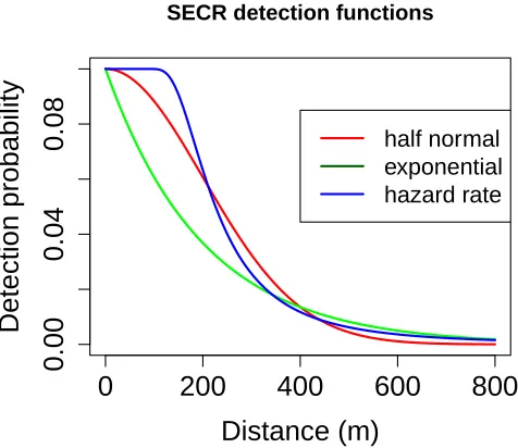
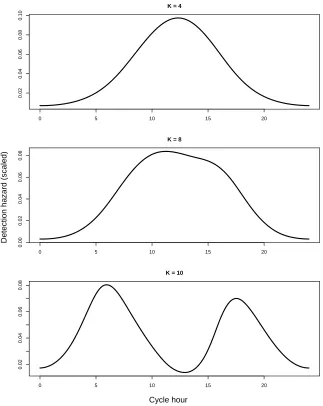
(13) List of Figures 1.1 1.2 1.3 2.1 2.2 2.3. 2.4. 3.1. 3.2 3.3 3.4. Camera trap survey sites within Cockscomb Basin Wildlife Sanctuary, Belize. . . . . . . . . . . . . . . . . . . . . . . . . . . . . . . . . . . . Study areas for the jaguar and possum analyses. . . . . . . . . . . . Example of a handwritten timing sheet with possum capture data that needed to be transcribed and formatted. . . . . . . . . . . . . . . . . Three different possible forms for the spatial detection function. . . . Standard cosine function with the number of radians in terms of π on the x axis. . . . . . . . . . . . . . . . . . . . . . . . . . . . . . . . . Three examples of possible detection hazard shapes that can be modelled using regression splines of increasing complexity. From top to bottom the degrees of freedom are 4, 8 and 10. . . . . . . . . . . . . Plots of 500,000 simulated first capture times from a hypothetical study lasting 56 hours and using three different underlying 24 hour hazards. The underlying hazards (blue) and the theoretical distribution of first capture times (red) are scaled appropriately and overlaid on the simulated times (grey). . . . . . . . . . . . . . . . . . . . . . Simulated movement for a single individual for a 90 day period in hourly steps, showing the number of times each cell is visited in the period and smoothed with a nonparametric smoother. . . . . . . . . . Four realisations from different Neyman-Scott distributions with density = 0.5 per ha. . . . . . . . . . . . . . . . . . . . . . . . . . . . . . Four realisations from different Neyman-Scott distributions with density = 2 per ha. . . . . . . . . . . . . . . . . . . . . . . . . . . . . . . Simulated density surfaces used in the linear, exponential and quadratic density scenarios for single-catch trap data. The vertical dashed red lines indicate the borders of the trap array. . . . . . . . . . . . . . . . xi. 8 10 10 18 36. 38. 39. 53 61 62. 63.

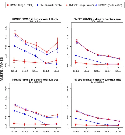
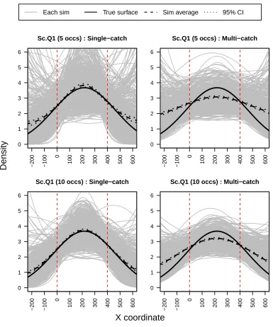
(14) LIST OF FIGURES 3.5 3.6 3.7 3.8 3.9 3.10. 3.11. 3.12 3.13 3.14 3.15 3.16 3.17 3.18 3.19. 3.20. Estimated density surfaces from the simulation scenario Sc.E1 for single-catch trap data with a constant hazard. . . . . . . . . . . . . Estimated density surfaces from the simulation scenario Sc.E2 for single-catch trap data with a constant hazard. . . . . . . . . . . . . Estimated density surfaces from the simulation scenario Sc.E3 for single-catch trap data with a constant hazard. . . . . . . . . . . . . Estimated density surfaces from the simulation scenario Sc.E4 for single-catch trap data with a constant hazard. . . . . . . . . . . . . Estimated density surfaces from the simulation scenario Sc.E5 for single-catch trap data with a constant hazard. . . . . . . . . . . . . Sampling distributions of the estimates for the slope in the exponential density model for both the multi and single-catch trap estimators for single-catch trap data with a constant hazard. . . . . . . . . . . . . Measures of model performance based on predicted density from the exponential density simulations for single-catch trap data with a constant hazard. . . . . . . . . . . . . . . . . . . . . . . . . . . . . . . . Estimated density surfaces from the simulation scenario Sc.Q1 for single-catch trap data with a constant hazard. . . . . . . . . . . . . Estimated density surfaces from the simulation scenario Sc.Q2 for single-catch trap data with a constant hazard. . . . . . . . . . . . . Estimated density surfaces from the simulation scenario Sc.Q3 for single-catch trap data with a constant hazard. . . . . . . . . . . . . Estimated density surfaces from the simulation scenario Sc.Q4 for single-catch trap data with a constant hazard. . . . . . . . . . . . . Estimated density surfaces from the simulation scenario Sc.Q5 for single-catch trap data with a constant hazard. . . . . . . . . . . . . Estimated density surfaces from the simulation scenario Sc.Q6 for single-catch trap data with a constant hazard. . . . . . . . . . . . . Estimated density surfaces from the simulation scenario Sc.Q7 for single-catch trap data with a constant hazard. . . . . . . . . . . . . Measures of model performance based on predicted density from the quadratic density simulations for single-catch trap data with a constant hazard. . . . . . . . . . . . . . . . . . . . . . . . . . . . . . . . Results from two of the single-catch trap simulations where the data are from non-constant density surfaces (exponential and quadratic) and the models specify a constant density. . . . . . . . . . . . . . . . xii. 71 72 73 74 75. 76. 77 78 79 80 81 82 83 84. 85. 89.

(15) LIST OF FIGURES 4.1. 4.2. 4.3. 4.4 4.5. 4.6. 4.7. 4.8. 4.9. 4.10 4.11 4.12. 4.13. Simulated density surfaces used in the exponential and quadratic density scenarios for proximity detectors. The vertical dashed red lines indicate the borders of the trap array. . . . . . . . . . . . . . . . . . . Histograms of simulated capture times from a survey with proximity detectors and a cosine detection hazard. The top panel collapses all captures (7,407 captures) into one cycle and the bottom panel plots the first ten cycles (798 captures). . . . . . . . . . . . . . . . . . . . Estimated hazard surfaces from the proximity detector simulation scenarios with both constant and non-constant density and a 24 hour cosine hazard. . . . . . . . . . . . . . . . . . . . . . . . . . . . . . . Estimated density surfaces from the proximity detector simulation scenarios Px.E1 and Px.Q1 with a 24 hour cosine hazard. . . . . . . . . Estimated hazard surfaces from the proximity detector simulation scenarios with constant density and a 24 hour spline hazard (K = 4 in the top panel and K = 8 in the bottom panel). . . . . . . . . . . . . Estimated density surfaces from the proximity detector simulation scenario Px.E1 with a 24 hour spline hazard (K = 4 in the top panel and K = 8 in the bottom panel). . . . . . . . . . . . . . . . . . . . . . . A 30 day (720 hours) hazard that repeats three times over the simulated study duration and a 90 day (2,160 hours) hazard with the same shape that does not repeat. . . . . . . . . . . . . . . . . . . . . . . . Estimated hazard surfaces from the simulation scenarios with an asynchronous spline hazard (K = 8) with a cycle length of either 30 days (top panel) or 90 days (bottom panel). . . . . . . . . . . . . . . . . . Estimated density surfaces from the proximity detector simulation scenario Px.E2 with an asynchronous spline hazard (K = 8) that has a cycle length of either 30 days (top panel) or 90 days (bottom panel). Detection hazard plots with a 24 hour cosine hazard and three 24 hour cyclic cubic spline hazards fitted to the jaguar data. . . . . . . . . . Assessing the goodness-of-fit of the estimated spline hazard from the best CT model to the jaguar capture times . . . . . . . . . . . . . . . Estimated hazard surfaces from the single-catch trap simulation scenarios with constant density and a 30 hour spline hazard (K = 4 in the top panel and K = 6 in the bottom panel). . . . . . . . . . . . . Estimated density surfaces from the single-catch trap simulation scenarios with exponential density gradients and a 30 hour spline hazard with K = 4. . . . . . . . . . . . . . . . . . . . . . . . . . . . . . . . xiii. 96. 99. 101 102. 104. 105. 107. 108. 109 113 114. 117. 118.

(16) LIST OF FIGURES 4.14 Sampling distributions of the estimates for the slope in the exponential density model for both the multi and single-catch trap estimators, for single-catch trap data with a time-varying hazard. . . . . . . . . . . 119 4.15 Measures of model performance based on predicted density from the exponential density simulations for single-catch trap data with a 30 hour cyclic spline hazard. . . . . . . . . . . . . . . . . . . . . . . . . 120 4.16 Estimated density surfaces from the single-catch trap simulation scenarios with quadratic density and a 30 hour spline hazard with K = 4. . . . . . . . . . . . . . . . . . . . . . . . . . . . . . . . . . . . . . 121 4.17 Measures of model performance based on predicted density from the quadratic density simulations for single-catch trap data with a 30 hour cyclic spline hazard. . . . . . . . . . . . . . . . . . . . . . . . . . . . 122 4.18 Detection hazard plots with three 24 hour cyclic cubic spline hazards fitted to the possum data. . . . . . . . . . . . . . . . . . . . . . . . . 125 D.1 Estimated hazard surfaces from the proximity detector simulation scenarios with exponential density and a 24 hour spline hazard (K = 4 in the top panel and K = 8 in the bottom panel). . . . . . . . . . . . 172 D.2 Estimated hazard surfaces from the proximity detector simulation scenarios with quadratic density and a 24 hour spline hazard (K = 4 in the top panel and K = 8 in the bottom panel). . . . . . . . . . . . . 173 D.3 Estimated density surfaces from the proximity detector simulation scenario Px.Q1 with a 24 hour spline hazard (K = 4 in the top panel and K = 8 in the bottom panel). . . . . . . . . . . . . . . . . . . . . . . 174 D.4 Estimated hazard surfaces from the proximity detector simulation scenarios with constant density and a 30 hour spline hazard (K = 4 in the top panel and K = 8 in the bottom panel). . . . . . . . . . . . . 175 D.5 Estimated hazard surfaces from the proximity detector simulation scenarios with exponential density and a 30 hour spline hazard (K = 4 in the top panel and K = 8 in the bottom panel). . . . . . . . . . . . 176 D.6 Estimated density surfaces from the proximity detector simulation scenario Px.E2 with a 30 hour spline hazard (K = 4 in the top panel and K = 8 in the bottom panel). . . . . . . . . . . . . . . . . . . . . . . 177 D.7 Estimated hazard surfaces from the proximity detector simulation scenarios with quadratic density and a 30 hour spline hazard (K = 4 in the top panel and K = 8 in the bottom panel). . . . . . . . . . . . . 178 xiv.

(17) LIST OF FIGURES D.8 Estimated density surfaces from the proximity detector simulation scenario Px.Q1 with a 30 hour spline hazard (K = 4 in the top panel and K = 8 in the bottom panel). . . . . . . . . . . . . . . . . . . . . . . D.9 Estimated density surfaces from the proximity detector simulation scenario Px.Q2 with an asynchronous spline hazard (K = 8) that has a cycle length of either 30 days (top panel) or 90 days (bottom panel). D.10 Estimated hazard surfaces from the single-catch trap simulation scenarios with constant density, a higher value for g0 (0.4), and a 30 hour spline hazard (K = 4 in the top panel and K = 6 in the bottom panel). D.11 Estimated hazard surfaces from the single-catch trap simulation scenarios with exponential density and a 30 hour spline hazard (K = 4 in the top panel and K = 6 in the bottom panel). . . . . . . . . . . . D.12 Estimated density surfaces from the single-catch trap simulation scenarios with exponential density gradients and a 30 hour spline hazard with K = 6. . . . . . . . . . . . . . . . . . . . . . . . . . . . . . . . D.13 Estimated hazard surfaces from the single-catch trap simulation scenarios with quadratic density and a 30 hour spline hazard (K = 4 in the top panel and K = 6 in the bottom panel). . . . . . . . . . . . . D.14 Estimated density surfaces from the single-catch trap simulation scenarios with quadratic density and a 30 hour spline hazard with K = 6. . . . . . . . . . . . . . . . . . . . . . . . . . . . . . . . . . . . . .. xv. 179. 180. 181. 182. 183. 184. 185.

(18) LIST OF FIGURES. xvi.

(19) List of Tables 2.1. Summary of the different models used in this research. Time formulation refers to the use of either a discrete-time (DT) model or a continuous-time (CT) model. . . . . . . . . . . . . . . . . . . . . . . .. 34. Model selection summary for the jaguar data. All models specify a constant density. . . . . . . . . . . . . . . . . . . . . . . . . . . . . .. 48. Estimates (and 95% confidence intervals) from the DT binary and the CT proximity detector models fitted to the male jaguar data with constant density specified and different behavioural effects. The best fitting models are marked in bold. . . . . . . . . . . . . . . . . . . . .. 49. 3.3. Movement model parameter values used in the movement simulations.. 54. 3.4. Relative bias (RB) of density and detection parameters estimated by the DT binary and the CT proximity detector models with a constant hazard. The data are simulated for a survey duration of T = 2,160 hours under the independence assumption with constant density and a constant hazard. . . . . . . . . . . . . . . . . . . . . . . . . . . . .. 55. Relative bias (RB) of density estimated by the DT binary and the CT proximity detector models with a constant hazard. All models specify a constant density. The data are simulated for a survey duration of T =2,160 hours with constant density and from an animal movement model that induces spatio-temporal correlation. . . . . . . . . . . . .. 57. Details of the different density surfaces used in the single-catch trap simulations. . . . . . . . . . . . . . . . . . . . . . . . . . . . . . . . .. 64. Details of the different Neyman-Scott clustered distributions used in the single-catch trap simulations. . . . . . . . . . . . . . . . . . . . .. 65. 3.1 3.2. 3.5. 3.6 3.7. xvii.

(20) LIST OF TABLES 3.8. 4.1. Coverage of the parameter and derived density estimates from the single-catch trap estimator for both the exponential and quadratic simulations, and for both 5 and 10 occasions of 24 hours. The Delta method was used to calculate the variance in the derived density estimates. . . . . . . . . . . . . . . . . . . . . . . . . . . . . . . . . . . .. 91. Details of the different density surfaces used in the proximity detector simulations. . . . . . . . . . . . . . . . . . . . . . . . . . . . . . . . .. 97. 4.2. Details of the different density surfaces used in the proximity detector simulations with the second and third asynchronous hazards. . . . . . 107. 4.3. Model selection summary for the jaguar data and the CT models with cyclic spline hazards for three different values of K. All models specify a constant density. . . . . . . . . . . . . . . . . . . . . . . . . . . . . 111. 4.4. Estimates (and 95% confidence intervals) from the CT proximity detector models with non-constant detection hazards fitted to the male jaguar data with constant density specified and different behavioural effects. The best model as indicated by AIC for each type of hazard is marked in bold and the best model overall is highlighted in orange. 112. 4.5. Model selection summary for the possum data and the CT models with cyclic spline hazards for three different values of K. All models specify a constant density. . . . . . . . . . . . . . . . . . . . . . . . . 126. 4.6. Estimates (and 95% confidence intervals) from the CT single-catch trap models with non-constant detection hazards fitted to the possum data with constant density specified and different behavioural effects. The best model as indicated by AIC for each type of hazard is marked in bold and the best model overall is highlighted in orange. . . . . . 127. 4.7. Model selection summary for the possum data and the DT multi-catch models for different ways of handling the “DG” events. All models specify a constant density. . . . . . . . . . . . . . . . . . . . . . . . . 128. 4.8. Estimates (and 95% confidence intervals) from the DT multi-catch trap estimator, for different ways of handling the “DG” events, fitted to the possum data with constant density specified and different behavioural effects. The best fitting model for each method of handling the trap failures is marked in bold. . . . . . . . . . . . . . . . . . . . 129 xviii.

(21) LIST OF TABLES B.1 Relative bias (RB) of density and detection parameters estimated by the DT multi and the CT single-catch trap estimators with a constant hazard. All models specify a constant density. The data are simulated for a survey duration of T = 120 or 240 hours with constant density and a constant hazard. . . . . . . . . . . . . . . . . . . . . . . . . . . B.2 Relative bias (RB) of density and detection parameters estimated by the DT multi and the CT single-catch trap estimators with a constant hazard. All models specify a constant density. The data are simulated for a survey duration of T = 120 or 240 hours from different linear density gradients and a constant hazard. . . . . . . . . . . . . . . . . B.3 Relative bias (RB) of density and detection parameters estimated by the DT multi and the CT single-catch trap estimators with a constant hazard. All models specify a constant density. The data are simulated for a survey duration of T = 120 or 240 hours from different exponential density gradients and a constant hazard. . . . . . . . . . . . . . . B.4 Relative bias (RB) of density and detection parameters estimated by the DT multi and the CT single-catch trap estimators with a constant hazard. All models specify a constant density. The data are simulated for a survey duration of T = 120 or 240 hours from different quadratic density surfaces and a constant hazard. . . . . . . . . . . . . . . . . . B.5 Relative bias (RB) of density and detection parameters estimated by the DT multi and the CT single-catch trap estimators with a constant hazard. All models specify a constant density. The data are simulated for a survey duration of T = 120 hours from various Neyman-Scott distributions (as determined by the µc and σc parameters) and a constant hazard. The DT models use 5 occasions of 24 hours. . . . . . . B.6 Relative bias (RB) of density and detection parameters estimated by the DT multi and the CT single-catch trap estimators with a constant hazard. All models specify a constant density. The data are simulated for a survey duration of T = 240 hours from various Neyman-Scott distributions (as determined by the µc and σc parameters) and a constant hazard. The DT models use 10 occasions of 24 hours. . . . . . . B.7 Relative bias (RB) of density and detection parameters estimated by the DT multi and the CT single-catch trap estimators with a constant hazard. All models specify a constant density. The data are simulated for a survey duration of T = 120 or 240 hours from various NeymanScott distributions with a higher value for µc (15) and a constant hazard. . . . . . . . . . . . . . . . . . . . . . . . . . . . . . . . . . . . xix. 146. 147. 148. 149. 150. 151. 152.

(22) LIST OF TABLES B.8 Relative bias (RB) of density and detection parameters estimated by the DT multi and the CT single-catch trap estimators with a constant hazard. All models specify an exponential density model. The data are simulated for a survey duration of T = 120 or 240 hours from different exponential density gradients and a constant hazard. . . . . 153 B.9 Relative bias (RB) of density and detection parameters estimated by the DT multi and the CT single-catch trap estimators with a constant hazard. All models specify a quadratic density model. The data are simulated for a survey duration of T = 120 or 240 hours from different quadratic density surfaces and a constant hazard. . . . . . . . . . . . 154 C.1 Relative bias (RB) of density and detection parameters estimated by the DT binary and the CT proximity detector models with a constant hazard and a 24 hour cosine hazard. All models specify constant density. The data are simulated for a survey duration of T = 2,160 hours with constant density and a 24 hour cosine hazard. . . . . . . . 156 C.2 Relative bias (RB) of density and detection parameters estimated by the DT binary and the CT proximity detector models with a constant hazard and a 24 hour cosine hazard. All models specify constant density. The data are simulated for a survey duration of T = 2,160 hours with a constant density of 4 per 100 km2 and a 24 hour cosine hazard with 3 levels for g0 . . . . . . . . . . . . . . . . . . . . . . . . . 157 C.3 Relative bias (RB) of density and detection parameters estimated by the DT binary and the CT proximity detector models with a constant hazard and a 24 hour cosine hazard. All models specify exponential density. The data are simulated for a survey duration of T = 2,160 hours from different exponential density gradients and a 24 hour cosine hazard. . . . . . . . . . . . . . . . . . . . . . . . . . . . . . . . . . . . 158 C.4 Relative bias (RB) of density and detection parameters estimated by the DT binary and the CT proximity detector models with a constant hazard and a 24 hour cosine hazard. All models specify quadratic density. The data are simulated for a survey duration of T = 2,160 hours from different quadratic density surfaces and a 24 hour cosine hazard. . . . . . . . . . . . . . . . . . . . . . . . . . . . . . . . . . . . 159 xx.

(23) LIST OF TABLES C.5 Relative bias (RB) of density and detection parameters estimated by the DT binary and the CT proximity detector models with a 24 hour cyclic cubic spline hazard with K = 4 or K = 8. All models specify constant density. The data are simulated for a survey duration of T = 2,160 hours with constant density and a 24 hour cyclic cubic spline hazard with K = 4 or K = 8. . . . . . . . . . . . . . . . . . . . . . . 160 C.6 Relative bias (RB) of density and detection parameters estimated by the DT binary and the CT proximity detector models with a 24 hour cyclic cubic spline hazard with K = 4 or K = 8. All models specify exponential density. The data are simulated for a survey duration of T = 2,160 hours from different exponential density gradients and a 24 hour cyclic cubic spline hazard with K = 4 or K = 8. . . . . . . . . . 161 C.7 Relative bias (RB) of density and detection parameters estimated by the DT binary and the CT proximity detector models with a 24 hour cyclic cubic spline hazard with K = 4 or K = 8. All models specify quadratic density. The data are simulated for a survey duration of T = 2,160 hours from different quadratic density surfaces and a 24 hour cyclic cubic spline hazard with K = 4 or K = 8. . . . . . . . . . 162 C.8 Relative bias (RB) of density and detection parameters estimated by the DT binary and the CT proximity detector models with a 30 hour cyclic cubic spline hazard with K = 4 or K = 8. All models specify constant density. The data are simulated for a survey duration of T = 2,160 hours with constant density and a 30 hour cyclic cubic spline hazard with K = 4 or K = 8. . . . . . . . . . . . . . . . . . . . . . . 163 C.9 Relative bias (RB) of density and detection parameters estimated by the DT binary and the CT proximity detector models with a 30 hour cyclic cubic spline hazard with K = 4 or K = 8. All models specify exponential density. The data are simulated for a survey duration of T = 2,160 hours from different exponential density gradients and a 30 hour cyclic cubic spline hazard with K = 4 or K = 8. . . . . . . . . . 164 C.10 Relative bias (RB) of density and detection parameters estimated by the DT binary and the CT proximity detector models with a 30 hour cyclic cubic spline hazard with K = 4 or K = 8. All models specify quadratic density. The data are simulated for a survey duration of T = 2,160 hours from different quadratic density surfaces and a 30 hour cyclic cubic spline hazard with K = 4 or K = 8. . . . . . . . . . 165 xxi.

(24) LIST OF TABLES C.11 Relative bias (RB) of density and detection parameters estimated by the DT binary and the CT proximity detector models with either a 30 day or 90 day cyclic cubic spline detection hazard with K = 4 or K = 8. All models specify the correct density surface. The data are simulated for a survey duration of T = 2,160 hours from different density surfaces with either a 30 day or 90 day cyclic cubic spline detection hazard with K = 4 or K = 8. . . . . . . . . . . . . . . . . . C.12 Relative bias (RB) of density and detection parameters estimated by the DT multi and the CT single-catch trap estimators with a 30 hour cyclic cubic spline hazard with K = 4 or K = 6. All models specify constant density. The data are simulated for a survey duration of T = 240 hours with constant density and a 30 hour cyclic cubic spline hazard with K = 4 or K = 6. . . . . . . . . . . . . . . . . . . . . . . C.13 Relative bias (RB) of density and detection parameters estimated by the DT multi and the CT single-catch trap estimators with a 30 hour cyclic cubic spline hazard with K = 4 or K = 6. All models specify constant density. The data are simulated for a survey duration of T = 240 hours with constant density, a 30 hour cyclic cubic spline hazard with K = 4 or K = 6, and a higher value for g0 (0.4). . . . . . . . . . C.14 Relative bias (RB) of density and detection parameters estimated by the DT multi and the CT single-catch trap estimators with a 30 hour cyclic cubic spline hazard with K = 4 or K = 6. All models specify an exponential density model. The data are simulated for a survey duration of T = 240 hours from different exponential density gradients and a 30 hour cyclic cubic spline hazard with K = 4 or K = 6. . . . C.15 Relative bias (RB) of density and detection parameters estimated by the DT multi and the CT single-catch trap estimators with a 30 hour cyclic cubic spline hazard with K = 4 or K = 6. All models specify a quadratic density model. The data are simulated for a survey duration of T = 240 hours from different quadratic density surfaces and a 30 hour cyclic cubic spline hazard with K = 4 or K = 6. . . . . . . . .. xxii. 166. 167. 168. 169. 170.

(25) Chapter 1 Introduction 1.1. Estimating animal density. Estimating population size is a crucial component of ecological research and conservation management (Silver et al., 2004; Dillon and Kelly, 2007; Gardner et al., 2009; Royle et al., 2009b; Ivan et al., 2013b). Capture-recapture (CR) methods are well established and have been used for several decades to fit both closed-population models that estimate abundance, and open-population models that estimate demographic vital rates such as survival and recruitment (Cormack, 1965; Jolly, 1965; Seber, 1965; White et al., 1982). Closed population CR models estimate animal abundance but animal density is a vital parameter in wildlife management and conservation (Buckland et al., 1993; Marques et al., 2013), and is often preferable to abundance since density estimates can be compared across space and time (Gerber et al., 2012; Ivan et al., 2013a). Furthermore there is often interest in understanding how and why density varies in space (Gaston, 2003). An estimate of density is obtained by dividing the estimate of abundance N by the size of the sampled area. In addition to demographic closure, conventional closedpopulation CR models assume geographic closure, an assumption which hardly ever holds (White et al., 1982; Royle et al., 2009a,b; Gardner et al., 2009; Gerber et al., 2012). Movement of animals results in the effective trapping area (ETA) being larger than the actual trapping area (also know as the “edge effect”), and leads to negative bias in detection probabilities and positive bias in abundance and density estimates (White et al., 1982; Williams et al., 2002; Karanth and Nichols, 1998; Royle et al., 2009b; Foster and Harmsen, 2012; Ivan et al., 2013b). It is widely acknowledged that it is difficult and usually problematic to estimate the ETA (Royle et al., 2009b; 1.

(26) CHAPTER 1. INTRODUCTION Gardner et al., 2009; Obbard et al., 2010; Gerber et al., 2012; Noss et al., 2012). Typically the ETA is estimated by adding a buffer to the sampling area that represents the additional area outside the trapping grid used by captured individuals. The size of this buffer is usually based on capture data from the trap array and approaches tend to use half the Mean Maximum Distance Moved (MMDM) as advocated by Dice (1938) (Karanth and Nichols, 1998; Karanth et al., 2004; Maffei et al., 2004; Silver et al., 2004; Maffei and Noss, 2008; Noss et al., 2012) though some also use full MMDM (Soisalo and Cavalcanti, 2006; Trolle et al., 2007; Obbard et al., 2010) or some variant of this (Dillon and Kelly, 2007; Gerber et al., 2012). MMDM type measures are viewed as a proxy for home range diameter but tend to underestimate home ranges since the movement data is truncated at the edge of the sampling array (Maffei and Noss, 2008; Obbard et al., 2010; Foster and Harmsen, 2012). When abundance is fixed and the area occupied by the population unknown, apparent density is a linear function of the assumed area. Hence the particular method used will affect density estimates and consequently this approach is not robust (Maffei et al., 2004; Dillon and Kelly, 2007; Maffei and Noss, 2008; Foster and Harmsen, 2012; Gerber et al., 2012). It is well established that using survey areas that are too small leads to inflated estimates of density (Maffei and Noss, 2008; Foster and Harmsen, 2012). Studies that compare radio-telemetry data with MMDM methods confirm that the latter underestimate the size of an animal’s home range (Dillon, 2005; Soisalo and Cavalcanti, 2006) unless the survey area is large (a factor of at least four) relative to the average home range size (Maffei and Noss, 2008) which is unlikely for wide-ranging animals. Furthermore these ad hoc boundary-strip methods do not incorporate uncertainty in the estimation of the sampling area and result in density estimates that assume the effective sampling area is known with certainty (Gardner et al., 2009; Obbard et al., 2010; Gerber et al., 2012). The advent of spatially explicit capture-recapture (SECR), or more briefly spatial capture-recapture (SCR), methods that incorporate spatial information on where captures are made resolves this problem. SCR models allow inference about the underlying point process that determines the locations of individuals thereby relaxing the assumption of geographic closure and directly estimating density without requiring an ad hoc ETA estimate (Efford, 2004; Royle and Young, 2008; Borchers and Efford, 2008; Royle et al., 2009a,b; Efford et al., 2009a). The addition of spatial information also means that SCR models are able to account for trap failure and spatially varying effort. SCR models embed a detection function in the observation process that depends on the distance between an individual’s activity centre and the detector location. 2.

(27) 1.2. CAPTURING IN CONTINUOUS-TIME Consequently SCR models recognise that individuals that tend to roam far from a particular detector will be less likely to be detected compared to those that are closer to the detector, and hence model individual heterogeneity in detection probability. SCR models are still relatively new but over the past few years have experienced rapid growth in both method development and application (Efford et al., 2009b; Gardner et al., 2010; Kery et al., 2011; Borchers, 2012; Foster and Harmsen, 2012; Borchers, 2016; Borchers and Marques, 2016). The inclusion of spatial information means that SCR models make use of more information in the data compared to non-spatial CR studies, and this is particularly beneficial when studying the type of species where small data sets are the norm. Recent studies that compare results from SCR models to those that use conventional CR techniques with ad hoc boundary strip methods confirm that the latter tend to underestimate the effective sampling area and overestimate density, and recommend the use of the spatially explicit methods to estimate density (Obbard et al., 2010; Gerber et al., 2012; Noss et al., 2012). Ivan et al. (2013b) used a range of simulations to compare the performance of the maximum likelihood SCR approach with MMDM methods and a method that uses telemetry data (Ivan et al., 2013a). They found that overall the SCR estimator was the most consistent and also the most robust to changes in parameter levels (for detection probability, number of occasions, and abundance). The maximum likelihood SCR outperformed the other methods when capture probability was low, and outperformed MMDM approaches in almost all cases except where the home range was highly asymmetric or elongated in which case the methods performed similarly.. 1.2. Capturing in continuous-time. The monitoring of secretive species that occur at low densities and range over wide areas has proven to be difficult (Kery et al., 2011; Goldberg et al., 2015). These characteristics exacerbate two central problems with sampling animal populations, namely being unable to survey the entire area occupied by the population and being unable to detect all individuals within the surveyed area (Karanth et al., 2006; Royle et al., 2009a). These sorts of species are also often of the highest conservation concern (Thompson, 2004; Stuart et al., 2004). Similar problems occur with species that are difficult to detect visually and difficult to trap. Technological advances in non-invasive sampling methods such as scat or hair collection for genetic analysis, camera trapping, and acoustic detection have led to new ways of “capturing” individuals that are particularly useful for species that are difficult to survey using more conventional methods (Carbone et al., 2001; Karanth 3.

(28) CHAPTER 1. INTRODUCTION et al., 2006; Dillon and Kelly, 2007; Gardner et al., 2010; Kery et al., 2011; Foster and Harmsen, 2012; Noss et al., 2012). Camera trap arrays in particular have become one of the most important tools for assessment and management of species that are hard to detect by other means (Rowcliffe and Carbone, 2008). Griffiths and van Schaik (1993) first used camera traps to survey elusive rainforest mammals and they recommended a CR framework to estimate abundance. Karanth (1995) then used camera traps to obtain photographic captures of tigers that were analysed in a traditional CR framework. This pilot study used two to three camera traps that were rotated over different sites, and was limited by a small sample of ten individuals and 31 captures. The photographic capture approach has become an important monitoring tool since Karanth and Nichols (1998) extended the initial study and estimated tiger densities at four different sites (Foster and Harmsen, 2012). The same approach has since been used for other species that are also individually identifiable from photographs, including felids, canids, ursids, hyaenids, procynoids, tapirids and dasypodids (Silver et al., 2004; Maffei et al., 2004; Soisalo and Cavalcanti, 2006; Trolle et al., 2007; Dillon and Kelly, 2007; Maffei and Noss, 2008; Balme et al., 2009; Gardner et al., 2010; Noss et al., 2012; Gerber et al., 2012) and are increasingly used with SCR methods. Data from camera trap surveys have also been used for studies on species richness (Tobler et al., 2008) and occupancy (Linkie et al., 2007). Cameras are almost always placed in optimal locations to maximise capture probabilities (Karanth, 1995; Karanth and Nichols, 1998; Karanth et al., 2004; Silver et al., 2004; Karanth et al., 2006; Soisalo and Cavalcanti, 2006; Foster and Harmsen, 2012). Doing so can result in non-random, biased placement if the locations are only optimal for a subset of the population (Foster and Harmsen, 2012). For cats in dense habitat these optimal locations are usually along trails (Gerber et al., 2012). Harmsen et al. (2010a) studied differential use of trails by different mammal species and found very few captures of jaguars and no captures of pumas at off trail locations. Furthermore all jaguars caught off trail were also captured by on trail cameras which suggests that placing cameras on trails should not lead to much bias, at least in the case of this population of jaguars. Photographic captures differ fundamentally from traditional physical captures in that they are continuously sampled and record the exact time of capture (Foster and Harmsen, 2012). Spatial and non-spatial application of classic CR typically involves physically capturing and marking individuals at discrete sampling occasions in time, and the survey process generates well-defined sampling occasions. But when there is no physical capture and release, as in the case of camera trap studies or acoustic CR surveys that record times of detection, there is no well-defined sampling occasion. 4.

(29) 1.3. CONTINUOUS-TIME MODELS In such cases, aggregating data into capture occasions introduces subjectivity (the occasion length chosen by the analyst) and discards some information (the exact times of capture). Summarizing the data from camera trap CR studies into discrete capture occasions imposes an artificial construction on the data for reasons of analytic convenience. It is always a better policy to find a statistical formulation that fits the data than to shoehorn the data into a form that fits statistical formulations that happen to be available. The tendency with camera trap data has been towards the latter, typically camera trap studies aggregate the data into sampling occasions so that the data are then suitable for analysis. This approach is not necessarily the best approach for SCR analysis of camera trap studies. CR methods typically assume independence across occasions (model Mb relaxes this assumption) and SCR methods also assume independence between traps, i.e. the probability of being caught at a particular trap is not affected by a capture elsewhere. In general, the only benefit to imposing the artificial construct of occasions on continuous data is to remove correlation in the capture times so that the independence assumption is not violated, although there may be cases in which discrete summary statistics by occasion are sufficient statistics. There is also likely to be little additional information in multiple captures in a short time (Royle et al., 2009a,b). However, binning the data into occasions does not allow the inclusion of continuous covariates (for example weather) and limits the potential inferences that can be made regarding underlying biological processes that occur in continuous-time (CT). Furthermore, the use of occasions often leads to the assumption of equal occasion lengths so that the interpretation of the capture probabilities are comparable across different periods. Such an assumption is questionable when factors like trap failure exist. It is common to aggregate the data into 24 hour periods (Maffei et al., 2004; Foster and Harmsen, 2012) which can lead to the so called “midnight problem” (Jordan et al., 2011) where an animal photographed either side of midnight counts as two encounters as opposed to only counting as one encounter when captured twice during the same day. If animals are most active around the cutoff then capture probability will be positively biased, and this is likely to be true for nocturnal cats. Capture histories that use daily occasions for low density animals also tend to have many zeros (Foster and Harmsen, 2012).. 1.3. Continuous-time models. CT models avoid the problems mentioned above but are far less developed compared to discrete-time (DT) models (Chao, 2001; Xi et al., 2007; Barker et al., 2014). The 5.

(30) CHAPTER 1. INTRODUCTION earliest CR CT models are probably those of Craig (1953) and Darroch (1958) that assume equal catchability for all individuals at all times, but have been extended to include individual heterogeneity (Boyce et al., 2001). Becker (1984) first established a counting process framework for CT models that uses a martingale estimator. His model allowed time variation in the intensity or λ parameter and most of the subsequent development in CR CT models extend his approach to come up with more general models (Becker, 1984; Yip, 1989; Becker and Heyde, 1990; Yip et al., 1995, 1999; Lin and Yip, 1999; Yip and Wang, 2002; Hwang and Chao, 2002). Most of these models do not estimate detectability and abundance simultaneously. Nayak (1988), Becker and Heyde (1990), Hwang et al. (2002) and Xi et al. (2007) developed maximum likelihood estimators (MLEs) and Chao and Lee (1993) developed a CT estimator based on sample coverage. More recently Barker et al. (2014) developed a CR model for the sampling of DNA fragments in CT. The authors link their model with the earlier CT models and show that the earlier models can be written in terms of probability distributions and modelled within a Bayesian framework. Like the other CT models mentioned above, this model is not parameterised in terms of density and does not include spatial information on detections. There is no consensus on the utility of CT estimators. Some authors conclude that the use of a DT model to analyze a CT dataset will bias estimates (Yip and Wang, 2002; Barbour et al., 2013) and can result in a loss of efficiency (Xi et al., 2007; Chao and Huggins, 2005); while others find no benefit over discrete-occasion estimators (e.g. Chao and Lee, 1993; Wilson and Anderson, 1995). Chapter 2 shows that Chao & Lee’s (1993) conclusion that capture times are uninformative about abundance does not hold in general.. 1.4. Single-catch traps. The majority of studies of small mammals use single-catch traps that catch and hold a single animal at a time (Efford et al., 2009a; Krebs et al., 2011; Gerber and Parmenter, 2015). The use of single-catch traps results in captures that are not independent and the likelihood for such models is complex. Efford (2004) used simulation and inverse prediction to fit single-catch trap models but the likelihood for such models remains to be developed under the discrete-occasion setup (Efford et al., 2009a; Royle et al., 2013c). This research began with a particular focus on data from camera traps but it soon became apparent that using a CT framework also facilitates the development of a single-catch trap estimator. 6.

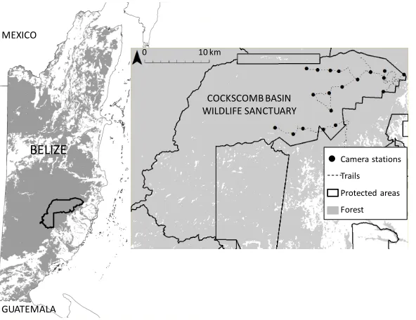
(31) 1.5. APPLICATIONS. 1.5. Applications. CR and SCR methods are increasingly used with camera traps for rare and elusive carnivores that are difficult to monitor with traditional methods (Dillon, 2005; Gerber et al., 2012), and camera traps yield CT capture data that are appropriate for CT models. The CT single-catch trap estimator that is developed in this research is appropriate for single-catch trap data with observed capture times. Jaguars are an example of a large carnivore that is notoriously difficult to study and possums are the type of small mammal that are often live-trapped with cage traps. The models that are developed in this research are therefore applied to two quite different datasets, one from a camera trap survey of jaguars and the other from a live-trapping study of possums where timing devices were fixed to the cages.. 1.5.1. Jaguars in Belize. Jaguars (Panthera onca) are near threatened and their global population is declining (Caso et al., 2008), and population monitoring is difficult because they occur at low densities, range widely and are elusive, often inhabiting thick habitat. Over the past decade, the challenge of detecting jaguars for population estimation has been facilitated by camera traps, following the work of Silver et al. (2004); however, reliable and robust density estimates of jaguars are rarely obtained (see Foster and Harmsen, 2012; Tobler and Powell, 2013). Study site and camera trapping of jaguars The Cockscomb Basin Wildlife Sanctuary in Belize encompasses 490 km2 of secondary tropical moist broadleaf forest at various stages of regeneration following anthropogenic and natural disturbance (for more details see Harmsen et al., 2010b). To the west, the sanctuary forms a contiguous forest block with the protected forests of the Maya Mountain Massif (≈ 5,000 km2 of forest). To the east the sanctuary is partially buffered by unprotected forest beyond which is a mosaic of pine savannah, shrub land and broadleaf forest, inter-dispersed with villages and farms. Jaguars are found throughout this landscape (Foster et al., 2010). There are 65 km of trails, all within the eastern part of the sanctuary (see Figure 1.1 and Figure 1.2). Few female jaguars were detected and since females have very different home ranges and possibly density, the analyses only use male detections. Male jaguars routinely walk the trail system and trail use overlaps extensively. Although they frequently leave the trails to move through the forest they are rarely detected offtrail by camera traps (Harmsen et al., 2010a). Nineteen paired camera stations 7.

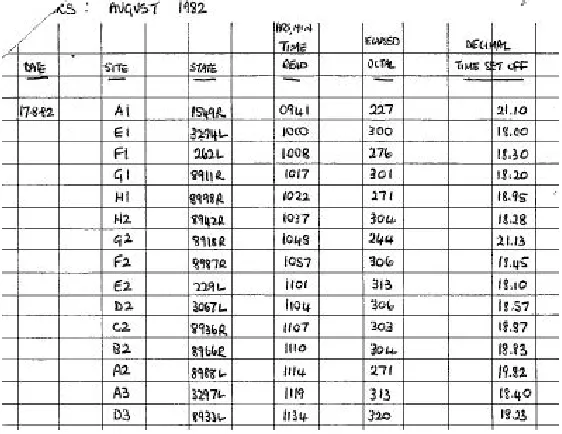
(32) CHAPTER 1. INTRODUCTION Figure 1.1: Camera trap survey sites within Cockscomb Basin Wildlife Sanctuary, Belize.. MEXICO 0. 10 km. COCKSCOMB BASIN WILDLIFE SANCTUARY. BELIZE. Camera stations Trails Protected areas Forest. GUATEMALA. (Pantheracam v3) were deployed along the trail network within the eastern basin and maintained for 90 days (April to July 2011) producing 207 captures of 17 individuals. Neighbouring stations had an average spacing of 2.0 km (1.1 to 3.1 km). Digital photographic data were downloaded every two weeks.. 1.5.2. Brushtail possums in New Zealand. Possums (Trichosurus vulpecula) were introduced to New Zealand in the nineteenth century to establish a fur industry (Efford and Cowan, 2004). Their selective browsing and predation on indigenous birds and invertebrates has caused them to become major pests (Campbell, 1990; Sadleir, 2000). Study site and trapping of possums The study site is in a mixed podocarp-hardwood forest in Orongorongo Valley on the North island of New Zealand (for more details see Efford and Cowan, 2004; Cowan and Forrester, 2012). Possums were live-trapped in a grid of wire mesh cage traps spaced 30 meters apart from each other that were baited with pieces of apple coated in flour and mixed with aniseed oil. The trapping ran for three consecutive days each month and traps were checked and reset daily. 8.

(33) 1.6. OBJECTIVE AND OVERVIEW The trapping grid is bounded to the north and west by the Orongorongo River. Apart from the river the habitat surrounding the trapping grid for several kilometers is similar to that covering the grid. Figure 1.2 shows the study area used in the possum analysis which has the river and the area across the river excluded as potential areas where activity centres could occur. Timing devices (accurate to within five minutes) were fitted to the door frames of the traps and were activated when the door closed. Occasionally other non-targeted species such as rats (Rattus rattus), mice (Mus musculus) and hedgehogs (Erinaceus europeus) triggered the traps. In these cases the timing devices still recorded the time that the trap was triggered and these events are referred to as “DG” events (door Down and bait Gone). In this population females breed once a year in May - June, young become independent during October to December, and juvenile dispersal occurs mostly from February to April but can happen from December to May. There may also be some additional movement of animals during the mating period (April-June) (Cowan, personal communication, 2015). In order to maintain the assumption of a closed population, the months of August, September and October (from 1982) are selected for analysis. The data were received in hand written timing sheets (see Figure 1.3) and were transcribed and formatted appropriately for analysis. From August to October 70 unique possums were trapped over 57 cage traps and there were 286 capture events. Trap saturation can be calculated as the average proportion of traps that are occupied at the end of an occasion, and in these data the average trap saturation was 58%.. 1.6. Objective and overview. The research presented here develops CT SCR likelihoods and MLEs which, unlike any existing CT models, are parameterised in terms of population density rather than abundance, and crucially, incorporate a model for (unobserved) individual activity centres. These models are obtained by formulating the SCR survey process as a type of recurrent event process, in which events are detections (see Cook and Lawless, 2007, for a comprehensive overview of recurrent event processes). The combination of recurrent event processes and CR methods was identified by Chao and Huggins (2005, p85) as “a fruitful area for future research”. Simulations are used extensively in this research as a tool for investigating how different estimators perform under different conditions. Chapter 2 presents the theory underlying the formulation of the CT SCR models. The first section provides methodological context by reviewing the existing DT SCR 9.

No results found