CARE, C. M. and CLEAVER, D. J. <http://orcid.org/0000-0002-4278-0098>
Available from Sheffield Hallam University Research Archive (SHURA) at:
http://shura.shu.ac.uk/869/
This document is the author deposited version. You are advised to consult the
publisher's version if you wish to cite from it.
Published version
CARE, C. M. and CLEAVER, D. J. (2005). Computer simulation of liquid crystals.
Reports on progress in physics, 68, 2665-2700.
Copyright and re-use policy
See
http://shura.shu.ac.uk/information.html
Computer simulation of liquid crystals
C M Care and D J Cleaver
Materials and Engineering Research Institute, Sheffield Hallam University, Howard Street, Sheffield, S1 1WB, UK
E-mail: [email protected],[email protected]
Abstract.
1. Introduction
In this article, we review molecular and mesoscopic computer simulations of liquid crystalline (LC) systems. Owing to their ability to form LC mesophases, the molecules of LC materials are often called mesogens. Following a scene setting introduction and a brief description of the key points of LC behaviour we first review the application of molecular simulation approaches to these mesogenic systems; we only consider bulk behaviour and do not report work on confined or inhomogeneous systems. This section is largely broken down by model-type, rather than area of application, and concentrates on the core characteristics of the various models and the results obtained. In contrast, in Section 4, we give relatively detailed descriptions of a series of recently developed lattice Boltzmann (LB) approaches to LC modelling and nemato-dynamics - following a period of relatively rapid development, a unifying review of this area is particularly timely. Finally, in Section 5, we identify a number of key unresolved issues and suggest areas in which future developments are likely to make most impact.
Note that we do not review results obtained using conventional solvers for the continuum partial differential equations of LC behaviour. Whilst it might legitimately be argued that the mesoscopic technique considered in this review, LB, is simply an alternative method of solving the macroscopic equations of motion for the LCs, this particular method is perhaps best thought of as lying on the boundary between macroscopic and molecular methods. Additionally, it is straightforward to adapt the LB method to include additional physics (eg the moving interfaces found in LC colloids); as such, a clear distinction can be drawn between the LB approaches reviewed in Section 4 and conventional continuum solvers.
Previous reviews of LC simulation include the general overviews by Allen & Wilson (1989) and Crain & Komolkin (1999) and a number of other works which concentrate on specific classes of model. For hard-particle models, the papers by Frenkel (1987) and Allen (1993) offer accessible alternatives to the all-encompassing Allen et al. (1993). Zannoni’s (1979) very early review of lattice models of LCs has now been significantly updated by Pasini et al. (2000a) in a NATO ARW proceedings (Pasini et al. 2000b) which contains some other useful overview material, while Wilson (1999) has summarised work performed using all-atom models. Finally, there are two accessible accounts of work performed using generic models - Rull’s (1995) summary of the studies that enabled initial characterisation of the Gay-Berne mesogen and the more recent overview by Zannoni (2001) which cogently illustrates subsequent developments and diversifications.
1.1. The role of computer simulation in liquid crystal research
Computer simulation is simply one of the tools available for investigating of mesogenic behaviour. It is, however, a relative newcomer compared with the many experimental and theoretical approaches available, and its role is often complementary; there is little to be gained from simulating a system which is already well characterised by more established routes. That said, appropriately focussed computer simulation studies can yield a unique insight into molecular ordering and phase behaviour and so inform the development of new experiments or theories. Most obviously, molecular simulations can provide systematic structure property information, through which links can be established between molecular properties and macroscopic behaviour. Alternatively, simulation can be used to test the validity of various theoretical assumptions. For example, by applying both theory and simulation to the same underlying model, uncertainties regarding the treatment of many-body effects in the former can be quantified by the latter.
At continuum length scales, LCs are characterised by a large number of experimentally observable parameters: viscosities, determined by the Leslie Coefficients; orientational elasticity, controlled by the Frank constants; substrate-LC orientational coupling, governed by anchoring coefficients and surface viscosities. Given a full set of these parameters, mesoscale simulations are now able to incorporate much of this complex behaviour into models of real devices. Thus, subject to the usual provisos concerning continuum models, these approaches are now starting to gain the status of design and optimisation tools for various LC device applications.
Before presenting the details of this review, we first ask the rather fundamental question - why perform computer simulations of LCs? LCs are fascinating systems to study because, like much of soft-condensed matter, their behaviour is characterised by the interplay of several very different effects which operate over a wide range of time- and length-scales. These effects range from changes in intra-molecular configurations, through intra-molecular librations to many-body properties such as mass flow modes and net orientational order to the fully equilibrated director field observed at the continuum length and time scales. The extent of the associated time- and length-scale spectra dictate that no single computer simulation model will ever be able to give a full ‘atom-to-device’ description for even the simplest mesogen. Moreover, since these different phenomena are, in general, highly coupled (eg intramolecular configurations are influenced, in part, by the local orientational order) they represent a multi-level feedback system rather than a simple linear chain of independent links. Thus, addressing each phenomenon with its own model and simply collating the outputs of a series of stand-alone studies will again fail to achieve a full description. In partial recognition of this, most of the methods and models currently used to simulate LCs seek to explore only a subset of the spectrum of behaviours present in a real system. In some cases, this pragmatic approach is entirely appropriate: for certain bulk switching applications, for example, a continuum description can prove perfectly adequate (explaining the popularity of Ericksen-Leslie theory) and the molecular basis of LCs can be neglected. Alternatively, a well defined generic model approach can provide the cleanest route to establishing relationships between molecular characteristics and bulk properties such as the Frank constants or the Leslie coefficients. Returning to the original question, then, we can reply that appropriately focussed simulation studies have certainly provided a sound understanding of many of the processes underlying bulk mesogenic behaviour and the operation of some simple switching devices.
The role of computer simulations in studying LCs is relatively well established; as noted above and shown in more detail in the following Sections, successful approaches have now been developed for many of the regions in the atom-to-device spectrum. As such, several of the fundamental problems in this field are now essentially solved. Given these achievements, it is now appropriate to raise the supplementary question - why continue to perform computer simulations of LCs? There is little of note to be gained by simply refining existing approaches and exploiting Moore’s law to incrementally enlarge the scope of, say, 3d bulk simulations of generic LC models of conventional thermotropic behaviour. Many of the outstanding challenges in LC science and engineering call, instead, for either predictive modelling, needed to make simulation an effective design tool for device engineers, or simulation methodologies capable of describing ‘butterfly’s wings’ problems, in which processes acting at molecular length-scales induce responses at the macroscale. Whilst addressing these classes of problem may require some development of new models, a more pressing need comes from the lack of adequate hybrid methodologies,i.e. two-way interfaces between existing classes of model. Indeed, the maturity of the field of LC simulation and the problems still posed to it mark it out as an ideal test-bed for moving established (but largely independent) models on to another level through the development of novel integrated simulation methodologies.
2. Materials and Phases
The LC phases are states of matter that exist between the isotropic liquid and crystalline solid forms in which the molecules have orientational order but no, or possibly partial, positional order. Particles which are able to form LC phases are called mesogenic, hence the term mesogen is used to refer to a molecule that forms a mesophase or LC phase. Typically, mesophases have some material properties associated with the isotropic liquid (ability to flow, inability to resist a shear) and others more commonly found in true crystals (long range orientational and, in some cases, positional order, anisotropic optical properties, ability to transmit a torque). The term LC actually encompasses several different phases, the most common of which are nematic and smectic; these are described at length in the classic texts dedicated to LCs (Chandrasekhar 1992, deGennes & Prost 1993, Kumar 2001) and in a recently published collection of some of the key early research papers (Sluckin et al. 2004).
[image:6.595.104.476.344.506.2]Most mesogens are either calamitic (rod shaped) or discotic (disc like); a sufficient (though not necessary) requirement for a substance to form a mesophase is a strong anisotropy in its molecular shape. Typically, calamitic mesogens contain an aromatic rigid core, formed from, eg , 1,4-phenyl or cyclohexyl groups, linked to one or more flexible alkyl chain(s). In families of LCs, the variants with short alkyl chains tend to be nematogens (mesogens that form nematic phases) while those with longer alkyl chains are smectogens (mesogens that form smectic phases).
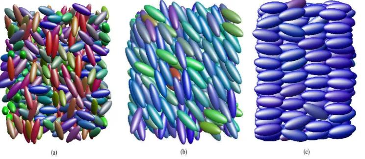
Figure 1. (a) Isotropic, (b) nematic and (c) smectic phases (configurations obtained from simulations performed using the Gay-Berne mesogen)
The nematic phase is the simplest LC phase and is characterised by long range orientational order but no long range translational order. In the nematic phase (Figure 1(b)), correlations in molecular positions are essentially the same as those found in an isotropic fluid but the molecular axes point, on average, along a common direction, the director ˆn. In the usual case of a nematic phase with a zero polar moment, the symmetry properties of the phase remain unchanged upon inversion of the director. If chiral molecules are used (or a chiral dopant is introduced), a cholesteric or chiral nematic phase can be obtained. The difference between this and the standard nematic phase is that in the former, the director twists as a function of position, but with a pitch which is much larger than molecular dimensions.
(a) 5CB (b) 8CB
Figure 2. 4-pentyl-4’-cyanobiphenyl (5CB) and 4-octyl-4’-cyanobiphenyl (8CB) molecules
The stability of LC phases can often be enhanced by increasing the length and polarisability of the molecule or by the addition of,eg, a terminal cyano group to induce polar interactions between the molecule pairs. Lateral substituents can also influence molecular packing. For example, incorporating a fluoro group at the side of the rigid core can enhance the molecular polarisability but disrupt molecular packing, leading to a shift in the nematic-isotropic (N-I) transition. Creating a lateral dipole in this way can also promote formation of tilted smectic phases and, in the case of chiral phases, give rise to ferroelectricity. Further details regarding the effects of various molecular features on nematic behaviour can be found in Dunmur et al. (2001).
The classic example of a room-temperature mesogen is then-cyanobiphenyl ornCB family shown in Figure 2. Here the rigid core is made of a meta biphenyl unit; at one end of this core is the flexible tail, an alkyl chain of n carbons (CnH2n+1), while at the other is the polar cyano head group. The
influence of the alkyl chain length is apparent from a comparison of the phase sequences for 5CB and 8CB.
5CB : Crystal23◦C
→Nematic35◦C
→Isotropic
8CB : Crystal21◦C→Smectic A32.5◦C→Nematic40◦C→isotropic
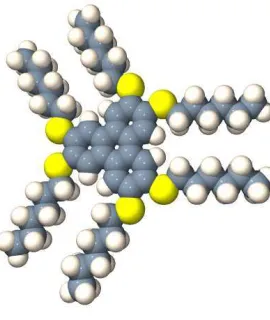
For molecules such as HHTT (Figure 3), in which one of the molecular axes is significantlyshorter than the other two, the alternative family of discotic phases can arise. Discotic mesogens typically have a core composed of aromatic rings connected in an approximately circular arrangement from which alkyl chains extend radially. In the discotic nematic phases, the director is the average orientation of theshortmolecular axes. As with the smectic phases, several types of columnar discotic arrangement have been suggested, the characterisation relating to column-column correlations and the relationship between orientational and positional symmetry axes. Again, though, distinguishing between these different columnar phases is generally beyond the capabilities of current simulation models.
Figure 3. Molecular representation of the HHTT molecule (2,3,6,7,11-hexahexylthio-triphenylene).
such as biaxial (Madsen et al. 2004, Acharya et al. 2004), and ferroelectric nematic phases and enhanced flexoelectricity.
Finally, before closing this Section, it is relevant to note that virtually all of the mesogenic materials used in practical applications are multi-component formulations, typically comprising a dozen or more molecule types. Broadly speaking, the prevalence of multi-component systems is explained by the relative ease with which they can be used to relocate phase transition points and selectively modify material properties. The issue of formulation has only recently become accessible to simulation studies, however.
3. Molecular simulations of Liquid Crystals
3.1. Molecular simulation techniques
The burgeoning field of molecular simulation underpins all of the work described in this Section and so a brief summary of its key components is appropriate. Due to obvious space constraints, a full overview is not possible, and we strongly recommend the standard texts (Allen & Tildesley 1986, Rapaport 1995, Frenkel & Smit 2002) to the interested reader. Here, we restrict ourselves to a brief discussion of the approaches adopted, with the intention of illustrating what is and what is not available on the molecular simulator’s palette.
Just as each experimental technique is restricted to a certain time- and length-scale window, so different simulation approaches are able to probe different sets of observables. As such, choice of appropriate model type(s) and simulation technique(s) is crucial in any project: this is driven by the scientific problem of interest and tempered by knowledge/understanding of the limitations imposed by, eg , the computational resources available and the range of applicability of the different models considered.
Once an interaction potential and the associated thermodynamic conditions have been decided upon, the task for the simulator is commonly to evolve the system configuration from its starting point to its equilibrium state. Once equilibrated, the objective becomes to generate a series of representative particle configurations from which appropriate system observables can be measured and averaged. If, as is often the case, only static equilibrium properties are required, a broad range of techniques can be used to perform these equilibration and production stages. By far the most common of these are molecular dynamics (MD) and Monte Carlo (MC) methods.
In an MD simulation, the net force and torque acting on each interaction site are used to determine the consequent accelerations. By recursively integrating through the effects of these accelerations on the particle velocities and displacements, essentially by applying Newton’s laws of motion over short but discretised time intervals, the micro-mechanical evolution of the many-body system can be tracked within an acceptable degree of accuracy. Since it mimics the way in which a real system evolves, an MD simulation can be used to calculate dynamic properties (such as diffusion coefficients) as well as static equilibrium observables. Its strict adherence to microscopic dynamics means, however, that in some situations (eg bulk phase separation) MD does not offer the most efficient route to the equilibrium state; in such situations, MC methods often prove preferable.
In an MC simulation, the microscopic processes (eg the particle moves) through which the simulated system evolves are limited only by the simulator’s imagination - in principle, any type of move may be attempted, though some will prove more effective than others. For example, in the case of phase separation raised above, particle identity-swap moves can be considered. Despite this free rein in terms of the attempted moves made, adherence to the laws of statistical mechanics is ultimately ensured through the rules by which these moves are either accepted or rejected. Essentially, these rules are imposed such that, once the system has equilibrated, there is a direct relationship between run-averaged observable measurements and the static properties of interest. Thus, while MC simulations routinely use random numbers in the generation of new configurations, the statistical mechanical framework within which these random moves are set ensures that any averages calculated are equivalent to those that would have been obtained using another equilibrium simulation method (such as MD).
Most molecular simulations of LCs, be they MD or MC, involve the translation and/or rotation of interaction sites, processes that are well described by the formalism of rigid-body mechanics (Goldstein et al. 2002). The mechanical scheme adopted depends on the symmetry and flexibility of the model used but can, in some cases, require the use of quaternions (Allen & Tildesley 1986) rather than the conventional direction cosine description. Additionally, the director constraint approach introduced by Sarman (1996) can prove a useful tool when using MD simulations to investigate long length-scale phenomena. Most LC simulations involve either bulk systems requiring 3-d periodic boundary conditions (PBCs) or some combination of PBCs and confining walls (in one or more direction), the latter usually being imposed as a static force field. While cubic simulation boxes are adequate for isotropic and nematic fluids, it has been shown (Dom´ınguez et al. 2002) that the pressure tensor can become anisotropic at the onset of smectic order unless the box length ratios are allowed to vary.
Calculation of the key orientational observables - the nematic order parameter and director - is commonly based on the order tensor methodology described in the appendix to Eppenga & Frenkel (1984), although an alternative method, based on long range orientational correlations (see (Zannoni 1979)), is useful in some situations. For systems in which small numbers of particles are available for order parameter calculations (eg when calculating order parameter profiles in confined systems) the systematic overestimation inherent in these standard methods can become problematic. In such situations, it can prove beneficial to compensate directly for this systematic effect (Wall & Cleaver 1997) or calculate run-averages of orientational order with respect to some box-fixed axis (eg the substrate normal). Procedures have also been established for the measurement of higher rank order parameters (Zannoni 2000) and phase biaxiality (Allen 1990).
distinguished by the non-zero bond-orientational order found in the latter (Halperin & Nelson 1998). For tilted smectics, where the director is of little use when determining the layer normal, alternative schemes have been developed for projecting out the in-plane and out-of-plane components ofg(r) (de Miguel et al. 1991b, Withers et al. 2000) and determining the direction of tilt.
3.2. All-atom simulations
Conventionally, molecular simulation is dominated by models based on psuedo-atomistic representations of the molecules found, experimentally, to display the relevant type of behaviour. In the field of LC phase behaviour, however, all-atom models do not dominate: instead, the various generic models described in Subsection 3.3 are far more prevalent.
While all-atom simulations of mesogenic molecules were first performed some 15 years ago, relatively little progress has been made since that time in terms of using such simulations to inform mesogenic phase behaviour. This appears somewhat surprising given the conclusion drawn from Wilson & Allen (1991)’s early simulations on all-atom systems, that 1ns is sufficient to establish nematic order. However, as evidenced in the more recent review (Wilson 1999), this time-scale has proven to be a serious underestimate. Indeed, a recent (and impressive) foray by the Bologna group into all-atom modelling of aminocinnamate systems, which employed run-lengths of over 50ns, concluded that order parameter stability could only be considered reliable when no significant drift was observed for 10ns (Berardi, Muccioli & Zannoni 2004). Sadly, this casts doubt on the thermodynamic stability of many of the previous all-atom simulations of bulk LC behaviour.
In addition to this considerable issue of the time-scales required to establish nematic stability in all-atom models, recent evidence suggests that a non-trivial system-size threshold also needs to be exceeded before qualitative temperature dependence of orientational observables (particularly the nematic order parameter) can be achieved. Thus, while Berardi, Muccioli & Zannoni (2004) were able to establish nematic stability in their very long runs, they failed to observe increasing nematic order with decrease in temperature in their simulations of 98-molecule systems. However, increasing system size to hundreds of molecules (ie thousands of atomic interaction sites)has been shown by recent studies,eg (McDonald & Hanna 2004, Cheung et al. 2004), to yield qualitatively correct temperature dependence of the order parameter. Even here, though, long-lived dependence on the choice of initial conditions can prove significant (McDonald 2002). Now that these issues are recognised, it is to be hoped that more progress will start to be made in this field through application of parallel MD approaches along with,eg, multiple timestep methods and efficient treatments of long-range interactions (Glaser 2000). Due to the uncertainties associated with the simulations performed to date with all-atom models, it is not appropriate to draw too many conclusions regarding the various model parameterisations employed. In the main, these have been based on parameter sets derived for liquid-state simulation (eg Amber), both with and without various electrostatic contributions. For the cyanobiphenyl family, for example, numerous alternative models have been derived (Picken et al. 1989, Cross & Fung 1994, Cleaver & Tildesley 1994, Yoneya & Iwakabe 1995, Clark et al. 1997, Lansac et al. 2001, Cacelli et al. 2002), through various combinations of standard force fields and explicit quantum chemical calculation. Despite this wealth of models, however, the computational difficulties raised above have conspired to prevent any thorough comparative studies from being performed. Thus, even for these much-studied cyanobiphenyl systems, there is no clear consensus as to which intramolecular components (eg detailed torsional potentials, partial charges, point dipoles and quadrupoles) are required for an all-atom model to successfully achieve quantitative agreement with experimental observations.
3.3. Generic models - their bases, uses and limitations
The use of generic LC models is founded on the notion that much can be learned about mesogenic behaviour without recourse to intimate molecular detail. This view is supported by theory, most obviously Onsager’s classic proof that shape anisotropy alone can be sufficient to induce nematic order (Onsager 1949). Also experimental work on a diverse range of systems (eg suspensions of tobacco mosaic virus, cylindical micelles, chromonic stacks and latex ellipsoids) has shown that LC order is exhibited by a range of non-molecular bodies with high shape anisotropies. Thus, the relatively slow rate of progress in all-atom simulations of LC systems has run in parallel with (and, arguably, motivated) the development and use of a series of simplified (or ‘generic’) models whichdo offer routes for the systematic investigation of explicit relationships between underlying model properties and bulk behaviour. Furthermore, many of these models have proved amenable to treatment by various analytical approaches (such as density functional and integral equation theories), so that direct comparison of simulation and theoretical results has become an increasingly common approach in the development of this field.
3.3.1. Lattice Models
The simplest generic model of LC behaviour is the lattice-based Lebwohl-Lasher model (Lebwohl & Lebwohl-Lasher 1972, Lebwohl & Lebwohl-Lasher 1973). In this, unit vector spins, sited at the vertices of a simple cubic lattice, are free to rotate about their centres of mass subject to interactions with their nearest neighbours. In its basic form, this interaction is the purely anisotropic, headless Maier-Saupe potential originally developed for use in molecular field theory (Maier & Saupe 1958, Maier & Saupe 1959, Maier & Saupe 1960). The Lebwohl-Lasher model ignores the particulate basis of LC ordering, coarse-graining, instead, to the level where each of the interacting spins should probably be considered as a volume element containing a locally-ordered cluster of molecules (Berggren et al. 2003). That said, other elements of its behaviour (eg the decay length of spin-spin orientational correlations (Fabbri & Zannoni 1986)) imply that the lattice spacing distance should be of the same order as a molecular length. Interestingly, Onsager’s description of the N-I transition, in which the orientational entropy sacrificed on entering the nematic phase is balanced by enhanced translational entropy is not applicable to Maier-Saupe-based approaches including the Lebwohl-Lasher and some related off-lattice models eg (Luckhurst & Romano 1981, Wei & Patey 1992b, De Luca et al. 1994). In fact, results obtained using these latter models demonstrate the veracity of Born’s (1916) original hypothesis that anisotropic dispersion interactions (allied with either no steric component or a spherically symmetric steric component) can also be sufficient to induce nematic order. Put another way, once such enthalpic free-energy contributions are introduced, the pure entropy-balancing Onsager picture can be subordinate to these additional terms.Early work performed using the Lebwohl-Lasher model identified a temperature-driven onset of orientational order resembling the N-I transition (Zannoni 1979). This was confirmed by a comprehensive study by Fabbri & Zannoni (1986) who, as well as locating the transition, showed that this very simple model shows a pretransitional divergence of orientational correlations on cooling from the isotropic phase. Subsequently, Zhang et al. (1992) employed histogram reweighting and finite-size-scaling techniques to confirm the transition to be weakly first order, and Cleaver & Allen (1991) examined the model’s orientational elastic constants. A more structural perspective on this collective orientational ordering behaviour of this system is given in Gonin & Windle (1997).
have also been used to incorporate additional anisotropy effects (Hashim & Romano 1999) and to investigate chiral (Memmer & Janssen 1998b, Memmer & Janssen 1998a) and dimer (Luckhurst & Romano 1997) systems. A number of Lebwohl-Lasher model variants have also been used to simulate and investigate biaxial nematic behaviour (Luckhurst & Romano 1980, Biscarini et al. 1995, Chiccoli et al. 1999, Romano 2004a, Romano 2004b).
This class system has also been used to investigate the properties of various two-component mixtures. The first work in this area studied the effects of low concentrations of fixed isotropic sites on the surrounding liquid crystalline matrix (Hashim et al. 1986). Subsequently, this model was developed to allow the isotropic sites to move around the system, and a wider range of relative concentrations was incorporated, allowing phase separation between isotropic and nematic regions (Hashim et al. 1990). More recently, Bates (1998) has incorporated isotropic terms into the interaction scheme so as to give control over the interfacial properties of the phase separated systems, while Memmer & Janssen (1999) have studied the effects of chiral additives. All-mesogenic mixtures have also been studied. Hashim et al. (1993) investigated the behaviour of rod-disk mixtures, particularly the balance between phase separation and biaxial phase formation. Also, Polson & Burnell (1997) performed an initial study of fractionation effects at the N-I transition of a binary calamitic mixture. These binary mixtures have now been thoroughly investigated by Yarmolenko (2003) who has also attempted some initial investigations of ternary systems.
3.3.2. Off-Lattice Generic Models
We now consider the range of LC models in which freely-translating particles are used to represent individual molecules. The earliest work in this area concentrated on molecular shape alone and employed models of rigid, hard anisotropic particles. This approach was justified by both Onsager’s proof that a purely steric systems can exhibit a density-driven N-I transition (Onsager 1949), and simulation work on simple fluid systems which had shown that molecule shape plays the main role in determining structural properties. We concentrate here on identifying some of the key early papers in this hard particle work before listing some of the more recent diversifications in this field. Following this, we review the use of generic LC models incorporating both attractive and repulsive components.Hard Particle Models
The earliest work on hard particle simulations of LCs was Veillard-Baron’s investigation of the behaviour of hard ellipsoid systems (Vieillard-Baron 1972). While this work saw the development of some key algorithms and analysis techniques, the simulations themselves were restricted to short run-lengths. Thus, it was not until these systems were revisited by Frenkel and co-workers using Perram and Wertheim’s formulation of the hard ellipsoid contact function (Perram et al. 1984, Perram & Wertheim 1985) that their full phase behaviour became established. The first tentative phase diagram for three dimensional hard ellipsoid systems, proposed by Frenkel et al. (1981), contained four different phases namely isotropic, nematic, plastic crystal and ordered crystal. A subsequent investigation by Frenkel & Mulder (1985) established the range of stability of these phases; specifically, calamitic nematic phases were found for particle elongations k ≥ 2.75, the transition density reducing with increased molecular elongation. A decade later, following some dispute of these results, Allen & Mason (1995) performed a study of their system-size dependence which confirmed the validity of Frenkel and Mulder’s phase diagram. An extension of this phase diagram was then produced by Camp, Mason & Allen (1996) who located the N-I coexistence densities precisely using Gibbs-Duhem integration techniques. Studies by Allen (1990) and Camp & Allen (1997) of a biaxial version of the hard ellipsoid model then showed it to form isotropic, nematic, and biaxial phases as well as confirming the discotic nematic behaviour originally found by Frenkel & Mulder (1985). Again, the N-I and discotic nematic-isotropic phase transitions were located using Gibbs-Duhem integration methods. The major conclusion to be drawn from these results is that the main prediction of Onsager’s theory, made in the limitk→ ∞, continues to hold at the intermediate values k & 3 that correspond to the elongations of common molecular mesogens.cylinder of length L and diameter D fitted with two hemispherical end-caps, so that k = 1 +L/D). This model is popular because its contact function, while still not given by a closed analytical expression, is more straightforward to calculate than that of the hard ellipsoid. This gives obvious computational advantages and makes comparison with theory more amenable - the hard spherocylinder was the model used by Onsager. Additionally, the spherocylinder resembles the shape of various colloidal mesogenic materials such as the tobacco mosaic virus (Zasadzinski & Meyer 1986, Dogic & Fraden 1997). There is no unique discotic equivalent of the hard spherocylinder; both cut-spheres (Veerman & Frenkel 1992) and short cylindrical segments (Bates & Frenkel 1998a) have been studied, however.
The first computer simulation on hard spherocylinders was again performed by Vieillard-Baron (Vieillard-Vieillard-Baron 1974) using elongations k= 2 and 3. This study did not find any LC phases since, as was shown subsequently, these are only stable for k ≥ 4.1; Vieillard-Baron did attempt to investigate a system with k = 6 (for which the nematic phase is stable) but was thwarted by the lack of computational resources available to him. Over a decade later, Stroobants et al. (1986) found that systems of perfectly parallel spherocylinders form a smectic A phase between the nematic liquid and crystalline solid. Subsequently, Veerman & Frenkel (1990) revisited Vieillard-Baron’s hard spherocylinder systems with full orientational freedom; studying particles with elongationsk∈[0 : 6]; these authors found isotropic, nematic and smectic A fluid phases. A more complete phase diagram was later proposed by McGrother, Williamson & Jackson (1996) which showed that askwas increased, the smectic A phase was stable for k ≥ 4.2 whereas the nematic phase required k ∼ 5. Bolhuis & Frenkel (1997) later refined this phase diagram and extended it up to the Onsager limit. From these studies the phase stability of the hard spherocylinder was established as :
• nematic : k= 1 +DL ≥4.7.
• smectic A :k= 1 + L D ≥4.1.
In addition to these hard ellipsoid and spherocylinder systems, a number of other hard-particle mesogens have been studied. One of the simplest of these, a rigid linear hard sphere chain (Whittle & Masters 1991), proved to be one of the most problematic: here, because of their non-convex shapes, the molecules proved poor at sliding past one another, leading to the development of metastable glassy states in the vicinity of the N-I transition. The tendency of these systems to become irretrievably interlocked was overcome by Williamson & Jackson (1998) through the use of reptation moves. Once orientationally ordered, this model proved to be reasonably well behaved, exhibiting a stable nematic region and undergoing a reversible nematic-smectic A transition. The related rattling-hard-sphere-chain model studied by Wilson & Allen (1993) proved immune to this glassy behaviour at the N-I transition, and gave an effective route by which to study the effect of molecular rigidity on phase properties. Models comprising sphere chains with rigid (linear) and flexible subunits (McBride & Vega 2002) were subsequently used to study the use of partial molecular flexibility to tune in and out various smectic phases. The use of flexible end-chains to enhance smectic phase stability had previously been established by van Duijneveldt & Allen (1997) using hard spherocylinders with simple 4-point-site chains at each end.
The HGO model has the considerable advantage over the hard ellipsoid that its contact function takes a relatively simple closed form. As well as making simulations easier to perform, this closed form allows the excluded volume of a pair of HGO particles to be calculated analytically (Velasco & Mederos 1998), so making direct comparison possible with second virial-based theories. The HGO shape parameter can also be extended and generalised, allowing for a variety of particle shapes and mixtures thereof to be simulated very efficiently. Since the majority of these generalisations have been employed in Gay-Berne-like 12-6 potentials, we defer a full listing to the following subsection. Here, we simply pick out the study by Barmes et al. (2003) of hard tapered or pear-shaped objects performed using of one of these generalised HGO models. Here, both nematic and bilayer smectic phases have been found, the latter remaining stable for axial ratios as low as k = 3.0, ie significantly lower than that the k= 4.1 required for hard spherocylinders to form a smectic. Hard particle models of bent-core systems, related to the banana-shaped molecules more recently found to yield biaxial nematic behaviour (Madsen et al. 2004, Acharya et al. 2004), have also been investigated. These studies, based on spherocylinder dimer models, have found isotropic, nematic and both para electric and antiferro-electic smectic A phases (Camp, Allen & Masters 1996, Lansac et al. 2003). The extension of this class of model to spherocylinder trimers arranged in a zig-zag shape has led to the observation of remarkably rich phase behaviour for a purely steric model: depending on the zig-zag angle, this model gives either columnar, smectic A or tilted smectic arrangements when expanded from a crystalline state (Maiti et al. 1958).
Hard particle models have also been used to investigate various mixture systems. For example, in systems of length bi-disperse parallel spherocylinders Stroobants (1992) found that, at high densitites, the smectic phase becomes unstable with respect to columnar order. Similar behaviour was observed in a subsequent study of polydisperse rods (Bates & Frenkel 1998b), although here the destabilisation of the smectic phase did not occur until the level of polydispersity was moderately high. Rod-disk mixtures of hard particles with conjugate asymmetries (ie elongationskand 1/k) have been used to investigate the balance, at near equimolar concentrations, between biaxiality and phase separation (Camp & Allen 1996, Camp et al. 1997), the latter being the only finding in an independent study of a similar system (Galindo et al. 2000). Also, mixtures of spheres and parallel spherocylinders have been shown to form a microphase separated lamellar phase (Koda et al. 1996, Dogic et al. 2000), whereas mixtures of hard sphere and freely rotating HGO ellipsoids can exhibit full phase separation at the N-I transition (Antypov & Cleaver 2003).
Before closing this subsection, we note another class of purely-repulsive model mesogens that has attracted some interest. These ‘soft repulsive’ systems, are all based, qualitatively at least, on the Weeks-Chandler-Anderson truncation of the Lennard-Jones potential (Weeks et al. 1971). Since the repulsions in these systems are finite, temperature becomes a significant thermodynamic variable. The extra complication associated with this increase in phase space is largely offset, however, by certain pragmatic advantages; due to their smoothly varying interactions, these systems are both well-suited to conventional (readily parallelisable) MD approaches and less prone to structural bottlenecks than their hard-particle equivalents. Furthermore, the intrinsically short range of their interactions makes them computationally efficient. While the results obtained for linear soft sphere chains (Paolini et al. 1993) and soft repulsive spherocylinders (Earl et al. 2001) are qualitatively indistinguishable from those of their hard-particle equivalents, Xu et al. (1999) have used an innovative bent-rod soft-sphere system to investigate onset of tilted smectic behaviour. Also, Andrienko et al. (2001) have exploited the highly efficient soft gaussian overlap model (which was actually first used by Kushick & Berne (1973)) to simulate the necessarily large volume of mesogenic solvent needed to examine the defect structures associated with various LC colloid systems - this type of model is, then, a good candidate for exploration of structural behaviours on length-scales up to one micron.
& Berne 1981), a single-site model in which the particle shape and interaction well depth can both be made anisotropic. The Gay-Berne model has arguably been the most successful and popular model for LC simulation to date; however, it also has a significant number of detractors. For this reason, we start this subsection by giving both a description of its basis and a critique of its limitations.
The standard Gay-Berne model has, at its core, Berne and Pechukas’ HGO shape parameter (Berne & Pechukas 1972)
σ(ˆrij,ˆui,ˆuj) =σ0
·
1−χ
2
½
(ˆrij·uˆi+ˆrij·ˆuj)2
1 +χ(ˆui·ˆuj)
+(ˆrij·uˆi−ˆrij·uˆj)
2
1−χ(ˆui·ˆuj)
¾¸−1/2
(1)
whereˆrij=rij/rij is a unit vector along the vectorrij=ri−rjbetween particles iandj and the unit
vectorsuˆiand ˆuj denote their orientations. Here,χ is a fully specified function of the particle length
to breadth ratiol/dand is given by
χ= (l/d)
2−1
(l/d)2+ 1. (2)
As is apparent from these expressions, in this original version of the model, particlesiandjare assumed to have both axial and head-tail symmetry. Simplified and generalised versions of equation(1) have been determined for the cases where, respectively, one of the particles is a small (Berne & Pechukas 1972) or large (Antypov & Cleaver 2004a) sphere or the axis lengths of particlesi andj are different from one another (Cleaver et al. 1996). The utility of these generalisations is that they give the shape parameter in a relatively simple closed analytical form. This makes them straightforward to implement in MD or MC simulation or in,eg , density functional or integral equation theories. More complex routes to the gaussian overlap shape parameter, based on on-the-fly matrix inversions, have been proposed and implemented for biaxial particles (Ayton & Patey 1995, Berardi et al. 1998, Berardi & Zannoni 2000). Gaussian overlap shape parameters, based on expansions of Stone functions (Stone 1978), have also been proposed (Zewdie 1998b) for the generation of alternative particle shapes. This expansion approach has been used to simulate tapered, or pear-shaped, particles (Berardi et al. 2001) and it appears a viable, if complex, route for the generation of lower-symmetry objects. For cylindrically symmetric objects, a parametric generalisation of equation(1) developed by Barmes et al. (2003) is a computationally efficient variant of Zewdie’s expansion approach. Furthermore, being based on the HGO mixture formalism of Cleaver et al. (1996), this parametric approach offers a natural route to the study of more exotic multi-component mixtures (eg pear shaped objects mixed with polydisperse rods).
Equation(1) reveals both the utility and the foibles of the Gay-Berne class of model: it gives the effective contact distance between particles i and j in a form which is analytically closed but which cannot be expressed as a simple sum of contributions from each of the two particles. Indeed, due to its gaussian overlap origins, the HGO contact distance is in fact non-additive (i.e. it does not satisfy the Lorentz-Bertholet mixing rule) and there is no formal definition of the single-particle volume. This apparent failing is, from a chemist’s perspective, actually quite reasonable - due to their intramolecular flexibiilty, real mesogenic molecules do not have additive contact functions or fixed excluded volumes either. Furthermore, the qualitative equivalence of the mesogenic behaviours of Gay-Berne (or HGO-based) fluids and those of hard-ellipsoid-based potentials indicates that the approximations involved in the former are quite reasonable when all that is being sought is understanding of generic phase behaviour. For situations where the ratio of the largest to the smallest particle semi-axis lengths grows too large, however, the issue of non-addivity becomes significant, and the fundamentals of the potential need to be addressed (see, eg , (Antypov & Cleaver 2004a, Barmes & Cleaver 2005)). Also, due to issues related to the orientation-dependent particle volume of gaussian overlap models, difficulties can arise if Gay-Berne-like interaction sites are used in coarse-grained models of specific LC molecules.
a reasonable fit to a linear arrangement of four Lennard-Jones sites. This resulted in the now widely used Gay-Berne potentialVGB expressed as
VGB = 4ǫ(uˆi,ˆuj,ˆrij)©R12−R6ª (3)
withR= σ0
r−σ(uˆi,uˆj,rij) +σ0
.
Here, the strength parameter is defined as
ǫ(uiˆ,ˆuj,ˆrij) =ǫ0ǫν1(ˆui,ˆuj)ǫ
µ
2(ujˆ ,ˆuj,ˆrij) (4)
with
ǫ1(uˆi,uˆj) =£1−χ2(ˆui·uˆj)2¤−
1
2 (5)
and
ǫ2(uˆi,uˆj,ˆrij) = 1−
1 2χ
′
"
(ˆrij·ˆui+ˆrij·ˆuj)2
1 +χ′(uiˆ ·ˆuj) +
(ˆrij·uˆi−ˆrij·ˆuj)2
1−χ′(uiˆ ·ujˆ )
#
. (6)
χ′ is the energy anisotropy parameter defined usingk′, the ratio of end-to-end and side-by-side well depths (ǫee andǫss, respectively). Thus,
χ′= k′ µ−1
−1
k′µ−1+ 1 (7)
k′ = ǫee ǫss
.
The behaviour of the Gay-Berne model can be tuned through modification of the four parameters k, k′, µ and ν. The most studied parameterisation, GB(k, k′, ν, µ) = GB(3,5−1,1,2), is that put
forward by Gay & Berne (1981) from their fits to linear arrays of Lennard-Jones sites. Preliminary simulations performed by Adams et al. (1987) using this parametrisation showed the model to be suitable for LC modelling and observed both isotropic and nematic phases. Subsequently, Luckhurst et al. (1990), using the slightly different parametrisation GB(3,5−1,2,1), found much richer phase
behaviour comprising isotropic, nematic, smectic A , smectic B and crystal phases. Independently of this, a thorough study of the originalGB(3,5−1,1,2) parameterisation by the Seville group identified
its liquid-vapour coexistence envelope (de Miguel et al. 1990), and showed that its fluid phase diagram also contains a region of smectic A stability (de Miguel et al. 1991a, de Miguel et al. 1991b, Chalam et al. 1991, de Miguel 1993). The parametrisationGB(3,5−1,3,1) was used by other groups (Berardi
et al. 1993, Allen, Warren, Wilson, Sauron & Smith 1996); while this gives the same isotropic, nematic and smectic phases as the previous parametrisations, the increased value of µ allows for a wider window of nematic stability. The substantially different parametrisationGB(4.4,39.6−1,0.74,0.8) was
introduced by Luckhurst & Simmonds (1993) in an attempt to use a model more closely related to real molecular mesogens. This parametrisation was obtained from fitting the Gay-Berne potential to an axial average of an all-atom representation of the p-terphenyl molecule. Subsequently, Bates & Luckhurst (1999) performed a thorough study using the parameterisationGB(4.4,20−1,1,1) and found
the model to exhibit isotropic, nematic, smectic A and smectic B phases in good agreement with the behaviour of such real mesogens. An investigation into the generic effects of the attractive part of the potential (de Miguel et al. 1996) showed the importance of attractive forces for the formation of smectic phases by ellipsoidal particles, layered phases being favoured by increase in 1/k′. A related study into the effects of molecular elongation, k, on the Gay-Berne phase diagram (Brown et al. 1998) showed significant changes, notably in the liquid-vapour coexistence region.
modified version of equation(3) and a similar system was revisited by Zewdie (1998a) as an application of his expansion-function approach to the shape parameter.
One of the most insightful recent findings from LC simulation has been Berardi & Zannoni’s (2000) discovery of a biaxial nematic phase arising from a combination of steric and dispersive interactions. Here, using Gay-Berne particles with moderate shape biaxiality, a biaxial nematic phase was successfully stabilised by enhancing attractions between the particle edges (rather than their faces). Other departures from uniaxial molecule shapes largely have their origins in Neal et al.’s (1997) use of 3-Gay-Berne-site assemblies to investigate triangular and zig-zag shaped mesogens. The former were subsequently simplified to Gay-Berne plus sphere models of pear-shaped particles (Stelzer et al. 1999, Billeter & Pelcovits 2000) with measurable flexoelectric coefficients. Following this, tapered variants of single-site Gay-Berne particles with appropriately tuned dispersive interactions were refined to the point where they yielded a ferroelectric nematic phase (Berardi et al. 2001, Berardi, Ricci & Zannoni 2004), behaviour which, at the time of writing, has yet to be achieved experimentally. Neal et al.’s (1997) zig-zag model, meanwhile, inspired a single-site mimic comprising Gay-Berne shape and well-depth functions aligned along separate axes (Withers et al. 2000). This internally rotated Gay-Berne model readily yielded tilted smectic phases on cooling from isotropic configurations. More recently, multi-site models have been developed for bent-core molecules. These include 2-site Gay-Berne models (Memmer 2000b, Johnston et al. 2002) and 7-site bi-linear arrays of Lennard-Jones sites (Dewar & Camp 2004). In the latter case, a tilted smectic phase has been observed for small and moderate core-core angles, but this may be associated with the preference of sphere chains to adopt staggered packing arrangements. The link between molecular and phase chirality has been investigated using generic models in a number of papers by Memmer (Memmer et al. 1993, Memmer 2000a, Memmer 2001). Using an alternative, less prescriptive, approach to the imposition of boundary conditions on such systems, Varga & Jackson (2003) have observed chiral pitch values much greater than the sample dimensions.
Simulations of bidisperse mixtures of calamitic Gay-Berne molecules have confirmed experimental findings that, even in well-mixed systems, more mesogenic particles have higher order parameters than their less mesogenic counterparts (Bemrose et al. 1997). Through Gibbs ensemble Monte Carlo simulations of such systems, Mills & Cleaver (2000) have also made direct measurements of compositional fractionation of LC mixtures at the N-I transition. This finding is related to the behaviour observed in simulations of associating LCs (McGrother et al. 1997, Berardi et al. 1999). Here, short particles, able to dimerise via attractive end-sites, exhibit strong increases in dimerisation with the onset of nematic order. The prospect of even more exotic associating behaviour has been raised by the range of structures observed in recent simulations of rod-sphere mixtures (Antypov & Cleaver 2004b). Finally, in this subsection, we note that a considerable body of work has been amassed investigating the effect of electrostatic dipole and quadrupole moments on mesogenic behaviour. In virtually all cases, such studies have involved incorporation of these electrostatic contributions into established generic hard and soft particle models. As noted by McGrother et al. (1998), however, the effects of dipoles, in particular, have proven to be strongly dependent on the details of their location and orientation on the host particles.
was found to be increased (McGrother, Gil-Villegas & Jackson 1996). For central transverse dipoles, enhanced stability of the smectic A phase was again observed, with the additional feature of some in-plane chain- and ring-formation by the transverse dipoles (Gil-Villegas et al. 1997b). Similar studies performed on dipolar Berne systems have drawn largely equivalent conclusions. Thus, for Gay-Berne systems with central longitudinal dipoles (Satoh et al. 1996a, Houssa et al. 1998, Houssa et al. 1999), enhanced smectic phase stability was observed, whereas the nematic was favoured on shifting the dipole to a terminal location (Satoh et al. 1996b). For some parameterisations of the latter system, the smectic phase was found to develop a bilayer structure (Berardi, Orlandi & Zannoni 1996, Berardi, Orlandi, Photinos, Vanarakas & Zannoni 1996). Central transverse dipoles were found to have little effect on the mesogenic behaviour of Gay-Berne systems (Gw´o´zd´z et al. 1997). However, multiple electrostatic moments have been shown to have significant effects. Specifically, by studying two outboard dipoles at various angles to the molecular axis, Berardi et al. (2003) determined systems able to form tilted smectic phases. Tilted smectic behaviour had previously been induced in Gay-Berne systems through the inclusion of longitudinal point quadrupole moments (Neal & Parker 1998, Withers et al. 2002, Withers 2003). For transverse central quadrupoles, conversely, Neal & Parker (2000) observed a significant increase inTN I, even for small quadrupole moments. At
larger quadrupole values, this study also observed cubic smectic arrangements rather than the usual smectic B behaviour.
4. Mesoscopic simulations
Although molecular simulation methods are becoming increasingly successful at predicting the behaviour of LC materials on microscopic scales, for many applications it is also important to be able to model their behaviour at much longer length and time scales. For example, simulations at length scales greater than 1µm and time scales greater than 1 ms will be required to model a display device. These length and time scales are inaccessible to molecular simulations and it is therefore necessary to employ either macroscopic or mesoscopic methods. The equations governing the dynamics of a nematic with fixed order parameter are well established; if the material parameters are well defined, either by experiment or molecular simulation, and the system being considered is relatively simple, analytical or standard numerical solutions of the macroscopic equations may be the most appropriate way to determine the behaviour of the material at long length and time scales scales (eg Leslie 1979, Stewart 2003). Finite element methods have also been used to determine the response of an LC system at the macroscale (eg Yoon et al. 2004, James et al. 2004). For nematics with a variable order parameter there are, as explained below, a number of choices for the governing equations; once again, these may be solved by standard numerical methods (eg Svensek & Zumer 2002). However such methods are not always appropriate. Thus, for example, near to interfaces they are normally unable correctly to model systems with weak anchoring.
In order to model more complex systems such as confined LCs or mixtures of LCs with isotropic fluids, an alternative approach is to use a mesoscopic simulation method, such as the lattice Boltzmann method (LB). Such methods have the potential benefit that the underlying physics can be built into the rules of the simulation method and the macroscopic behaviour is then emergent. In addition to providing an efficient simulation scheme, the approach has the merit of providing insight into the origin of the macroscopic behaviour and may also provide a route to bridging the length scales from the microscopic to macroscopic. However a successful paradigm for bridging from molecular to macroscopic length scales has yet to be developed.
nematic LCs (Care et al. 2000, Denniston et al. 2001a, Denniston et al. 2004, Care et al. 2003, Spencer & Care 2005) and in the remainder of this section we review these methods and their applications. As far as the authors are aware, no attempt has been made to develop LB methods for any other LC mesophases. We should mention in passing that the LB method is able to model other phases of complex fluids; for example, LB models of amphiphilic systems have been able to to recover the gyroid phase (Gonzalez-Segredo & Coveney 2004). We note that Levine et al. (2005) have recently reported the use of DPD to model nematic and smectic phases; however the approach they use is closer the molecular simulations reported in Section 3 than the mesoscale approach which is the focus of this section.
We begin by reviewing the various macroscopic formalisms which have been employed as the target for the LB schemes. Rather than impose a single unified notation, we have adopted in each section the notation used in the appropriate literature. Although this has the consequence that the same physical quantity is sometimes described by different symbols, the reader should find the transition to the literature is achieved more readily.
4.1. Macroscopic equations for nemato-dynamics
The first choice which must be made in modelling a nematic LC is whether the order parameter can be considered to be essentially constant. For many systems this is a reasonable approximation and the Ericksen-Leslie-Parodi formalism (eg deGennes & Prost 1993, Chandrasekhar 1992, Stewart 2003) is a commonly used series of equations for such systems. Care et al. (2000) developed an LB method based on the ELP equations.
However, in many systems the spatial and temporal variation of the order parameter is important; for example, in the presence of defects, near to substrates or in shear-flows when the LC is close to the nematic-isotropic transition temperature. If the order parameter is allowed to vary, there are a number of different presentations of nematodynamics, with perhaps the earliest work by Hess (1975). A recent paper by Sonnet et al. (2004) using arguments based on Rayleigh’s dissipation function (eg Vertogen & de Jeu 1988) provides the basis upon which the variety of schemes with a variable order parameter may be compared.
The variable order parameter schemes are more straightforward to adapt to an LB formalism and the two approaches which have been used as the basis of LB nemato-dynamics are due to Qian & Sheng (1998) and Beris & Edwards (1994). The latter work is closely related to that of Olmsted & Goldbart (1990) which was also influenced by the work of Doi (1981) and Kuzuu & Doi (1983) on polymer rheology.
4.1.1. Constant order parameter: Ericksen-Leslie-Parodi formalism
If the order parameter is assumed to be constant throughout the system, the most usual form of the macroscopic equations are the Ericksen-Leslie-Parodi (ELP) equations of nematodynamics for an incompressible fluid although there is an alternative ‘Harvard’ formalism (deGennes & Prost 1993). These equations may be summarised as follows∇αvα= 0 (8)
Dvβ
Dt =∂ασαβ (9)
hα =γ1Nα+γ2nβAβα (10)
where
Nα=
Dnα
Dt −εαβγωβnγ (11)
The first two equations are the equations of continuity (8) and momentum evolution (9). Equation (10) may be considered to be an equation controlling the evolution of the director,nα. In these equations,
velocity gradient tensor and ωα = 12εαβγ∂βvγ is the fluid vorticity. The fieldhα(x, t) is a ‘molecular
field’ which mediates the effects of (i) the Frank elastic energy and (ii) the effect of any external applied magnetic or electric fields. In theone constant approximationin which the three Frank elastic constants are assumed to be equal to a single constant,K, the molecular field becomes
hα=K∂β∂βnα+χa(H.n)Hα (12)
where, for example, Hα is the external magnetic field and χa is the anisotropy in the susceptibility.
The viscous part of the stress tensor for a nematic may be written in the form
σ′
αβ= (α2nαhβ+α3hαnβ)/γ1+α1nαnβnγnδAγδ+α4Aαβ
(α5−α2γ2/γ1)nαnγAγβ+ (α6−α3γ2/γ1)nβnγAγα (13)
where
γ1=α3−α2 (14)
γ2=α6−α5=α2+α3 (15)
The latter relationship due to Parodi embodies the Onsager’s reciprocal relations for irreversible processes (eg (Chandrasekhar 1992))
4.1.2. Variable order parameter: Beris-Edwards formalism
If the order parameter cannot be assumed to be a constant, the formalism of nemato-dynamics is normally written in terms of evolution equations for the pressure, velocity, and a tensor order parameter, Qαβ. This latter quantity whichmay be written as
Qαβ=< mαmβ−
1
3δαβ> (16)
wheremαis a unit vector defining the orientation of an individual molecule and<>denotes an average
over all the molecules in the system. For a nematic with uniaxial symmetry,
Qαβ=S(nαnβ−
1
3δαβ). (17)
However, in general it must be assumed that the system will exhibit biaxiality; this is particularly important near to walls or defects.
In this section we present the equations of the Beris & Edwards’s (1994) formalism and essentially follow the notation adopted by Denniston et al. (2001a); in the subsequent section we present the Qian & Sheng (1998) formalism. It should be noted that the Beris-Edwards and Qian-Sheng equations reduce to the ELP formalism in the limit that the order parameter becomes independent of time and position. However, Sonnet et al. (2004) show that the two schemes differ in the terms which are included in the dissipation function.
In the Beris-Edwards scheme, the evolution equation forQαβ(≡Q) is
DQ
Dt −S(W,Q) = ΓH (18)
where Γ is a rotational diffusion constant. The first term on the left hand side is the convective derivative forQand the second term couples the velocity gradient tensorWαβ=∂βuα and the order
tensor. To lowest order inQthis is given by
S(W,Q) = (ξA+Ω)(Q+I
3) + (Q+
I
3)(ξA−Ω)−2ξ(Q+
I
3)Tr(QW) (19) where A = (W+WT)/2 is the symmetric, and Ω = (W−WT)/2 is the antisymmetric, velocity gradient tensor. We note thatΩ is related to the vorticity through Ωαβ=−εαβγωγ. The parameterξ
field, H, controls the relaxation to equilibrium and is derived from appropriate moments of the free energy,F,
H=−δF
δQ+ I
3Tr δF
δQ. (20)
If the free energy is given by
F=
Z
d3r{a
2Q
2
αβ−
b
3QαβQβγQγα+ c 4(Q
2
αβ)2+
K
2(∂αQβγ)
2}, (21)
The first three terms are the standard Landau-deGennes free energy which controls the nematic-isotropic phase transition and the equilibrium of the nematic in the absence of gradients in the order parameter. The last term is the elastic free energy in the one constant approximation. The molecular field derived fromF is
H=−aQ+b(Q2−I
3TrQ
2)−cQTrQ2+K∇2Q (22)
The fluid momentum obeys the Navier-Stokes type equations (8) and (9) with the stress tensor, σαβ
composed of a symmetric component
σs
αβ= −P δαβ+ηAαβ−ξHαγ(Qγβ+
1
3δαβ)−ξ(Qαγ+ 1
3δαγ)Hγβ
+ 2ξ(Qαβ+
1
3δαβ)QγεHγε−∂βQγε δF
δ∂αQγε
(23)
and an antisymmetric component
σαβa =QαγHγβ−HαγQγβ (24)
and the pressure is taken to be
P=ρT −K
2(∇Q)
2
(25)
In equation (23),η is the parameter equivalent to the isotropic viscosity α4 of the ELP theory.
4.1.3. Variable order parameter: Qian-Sheng formalism
An alternative formalism for the flow of a nematic LC with a variable scalar order parameter is due to Qian & Sheng (1998). It is important to note that Qian & Sheng (1998) employ a slightly different definition of the order tensor to that defined in equation 16. Hence they essentially defineQαβ=<
1
2(3mαmβ−δαβ)> (26)
and for a nematic with uniaxial symmetry this gives
Qαβ=
S
2(3nαnβ−δαβ). (27)
The definitions given by equations 16 and 26 both give a traceless tensor but the eigenvalues are not identical. The two governing equations of the Qian & Sheng scheme are the momentum evolution equation.
ρDtuβ=∂α(−P δαβ+σαβd +σ f
αβ+σvαβ) (28)
and the order tensor evolution equation
JQ¨αβ=heαβ+hvαβ−λNδαβ−εαβγλNγ (29)
where he
αβ (hvαβ) is the elastic (viscous) molecular field. The quantities λN and λNα are Lagrange
multipliers which impose the constraints that the order tensor,Qαβ, is symmetric and traceless.
& Prost 1993). In equations (28) and (29), Dt =∂t+uµ∂µ is the convective derivative and P is the
pressure in the nematic phase. σv
αβ is the viscous stress tensor,
σαβv =β1QαβQµνAµν+β4Aαβ+β5QαµAµβ+β6QβµAµα+
1
2µ2Nαβ−µ1QαµNµβ+µ1QβµNµα (30) where Aαβ = 12(∂αuβ+∂βuα) is the symmetric velocity gradient tensor andNαβ is the co-rotational
derivative defined by Nαβ = ∂tQαβ+uµ∂µQαβ−εαµνωµQνβ −εβµνωµQνα with ωµ being the fluid
vorticity. In equation (30),σd
αβ is the distortion stress tensor
σd αβ=−
∂fN
∂(Qµν, α)
Qµν, β (31)
where Qαβ,γ ≡∂γ(Qαβ) and σfαβ is the stress tensor associated with an externally applied field. The
bulk elastic molecular field is given by
heαβ=−
∂fN
∂ Qαβ
+∂µ
∂fN
∂(Qαβ, µ)
(32)
where the free energy density of the bulk nematic, fN, is given by a Landau-deGennes expression of
the form
fN =fN h+fN g (33)
where the homogeneous contribution,fN h, is given by
fN h= 1 2(αFQ
2
µν−βFQµνQντQτ µ+γF(Q2µν)2) (34)
and the gradient contribution,fN g, is given by
fN g= 1 2(L1Q
2
µν,τ+L2Qµν,νQµτ,τ) (35)
Using this form of the free energy the bulk molecular field, equation (32), is given by
heαβ=L1∂µ2Qαβ+L2∂β∂µQαµ−αFQαβ+ 3βFQαµQβµ−4γFQαβQ2µν (36)
The expressions (32) to (36) are essentially equivalent to equations (20) to (22) for the Beris-Edwards scheme. However, the free energy (21) only recovers the one constant approximation for the elastic constants, whereas that used by Qian-Sheng allows for two independent elastic constants defined in terms ofL1 andL2. In order to recover fully independent elastic constants, higher order terms in the
gradients ofQαβ must be included in either (21) or (35) for the free energy.
4.2. The lattice Boltzmann method for liquid crystals
We now discuss the application of the LB method to the modelling of liquid crystals. A short review of the LB method for isotropic fluids is given in Appendix A.
simulation can yield all the required coefficients; however there remain unresolved technical problems concerning the correct method to extract all the required information from the simulations. Theoretical work has been undertaken to derive the Leslie coefficients from molecular properties eg (eg Kuzuu & Doi 1983, Osipov & Terentjev 1989) using statistical mechanical arguments.
Given the complexity of the relationship between the molecular behaviour and the macroscopic coefficients, the approach to developing a LB scheme for the nematic phases has adopted a top down philosophy in which an LB scheme is designed to recover the required macroscopic equations rather than require the macroscopic equations to be emergent from some simplified mesoscopic dynamics. In order to adapt the LB method to represent a nematic LC it is necessary to add additional degrees of freedom to the LB densities in order to carry information about orientational order; the LB densities must not only transport mass and momentum information between sites, but also information about the orientational order of the fluid elements and the order parameter of the nematic. The schemes which are developed must then recover the equations associated with an appropriate macroscopic description of the nematic LC.
There have been essentially four approaches to this problem. Care et al. (2000) recovered the ELP equations using a scheme in which the momentum density fi is augmented by a second Boltzmann
equation for the propagation of a (two dimensional) vector which carries the order information. Denniston et al. (2001a) recover the Beris-Edwards equations by introducing a second Boltzmann equation which controls the evolution of a tensor order parameter; in the third approach (Care et al. 2003) also propagate a tensor density. Apart from the different target macroscopic equations, perhaps the principal difference between the latter two approaches lies in the way in which the coupling between the director and flow fields is achieved. In the approach of Denniston et al. this coupling is achieved by (i) modifications to the equilibrium distribution function and (ii) forcing terms, principally to introduce the antisymmetric components to the stress tensor. Care et al. (2003) achieve the coupling through (i) anisotropic scattering and (ii) forcing terms. In the most recent work by the latter group (Spencer & Care 2005) the forcing terms is used to introduce all the coupling. The methods of Denniston et al. (2004) and Spencer & Care (2005) appear to be of equivalent numerical complexity. One might argue that the equilibrium distribution function of a nematic is intrinsically isotropic for a real nematic but within the LB method the inclusion of physical phenomena through forcing or through the equilibrium distribution function are essentially equivalent, the difference perhaps being a matter of taste. In this review we only describe the method of Denniston et al. (2004) (Section 4.2.3) and the method of Spencer & Care (2005) (Section 4.2.4).
An important problem that needs to be considered when developing lattice Boltzmann schemes is the widely differing time and length scales associated with the macroscopic parameters; ie the momentum, the order parameter and the director (eg Qian & Sheng 1998). The order parameter changes on the shortest time scale; this is typically of the order of 0.1µs and over length scales which may be as short as a few nm. The time scale taken for the director to equilibrate depends upon the size of system being considered, but for typical devices sizes of 10µm it may take of the order of a second whereas the time taken for the velocity to come to steady state may be of the order of 1µs; this is consistent with a typical device Reynolds number of the order of 10−6. Handling these large differences
in time scale is a particular challenge when, for example, modelling switching in a real device geometry. One approach is to run the LB at the shortest time scale and completely resolve all the dynamics, but this is computationally very inefficient and it therefore preferable to operate the LB solver for the momentum on a different time scale to that for the director field. This is equivalent to the approach which is adopted with conventional solvers (eg Svensek & Zumer 2002). Care must also be taken to correctly recover the dynamics of the order parameter and this is an area of current research.