A New Method to Determine the Grid Directions in Reservoir Numerical Simulation

(1)

ISSN Print: 2156-8359

DOI: 10.4236/ijg.2018.912041 Dec. 28, 2018 680 International Journal of Geosciences

A New Method to Determine the Grid Directions

in Reservoir Numerical Simulation

Ming Li

1

, Luyi Tong

1

, Xiaodong Peng

1

, Guiping Nie

2

, Yan Lu

1*

1_{Zhanjiang Branch of CNOOC Limited, Zhanjiang, China}

2_{Engineering Technology Company of CNOOC Energy Technology & Services Limited, Zhanjiang, China}

Abstract

Grid direction selection and grid size design are two important elements that need to be considered in the grid direction design in reservoir numerical si-mulation. Reservoir engineers normally utilize geological data (such as the distribution of fractures, low permeability zones, faults and major stress) and simulation experiences to design the grid direction of simulation model qua-litatively. The research of the paper indicates that the key to determine the grid direction is to determine the principal permeability direction. Under the circumstances of few static materials, a new grid direction determination method has been developed by using field data (well location map and in-ter-well permeability) on the bases of Darcy’s law and tensor analysis theory. The grid direction of WZ11-7 Oilfield simulation model has been determined using four production wells and two production zones (L1 and L3) in WZ11-7-2

well group, the results are in conformity with the geological studied major stress. Therefore, this method can give insights into the numerical simulation study.

Keywords

Reservoir Numerical Simulation, Grid Direction, Black Oil Model, Permeability Anisotropy, Tensor Analysis

1. Introduction

Grid direction selection and grid size design are quite important, and should be considered in reservoir numerical simulation. Common grid direction selection should follow the following principles [1]: 1) grid direction should be consistent with the regional boundary (oil and gas, oil-water boundary lines, fault lines, re-servoir pinch lines, well networks, or structural symmetry lines) and well pattern direction as far as possible; 2) grid direction should take into account reservoir nature, namely, the coordinate system should be parallel (or perpendicular) to

How to cite this paper: Li, M., Tong, L.Y., Peng, X.D., Nie, G.P. and Lu, Y. (2018) A New Method to Determine the Grid Direc-tions in Reservoir Numerical Simulation. International Journal of Geosciences, 9, 680-687.

https://doi.org/10.4236/ijg.2018.912041

Received: November 19, 2018 Accepted: December 25, 2018 Published: December 28, 2018

(2)

DOI: 10.4236/ijg.2018.912041 681 International Journal of Geosciences

the main axis of permeability, or approximately in line with the direction of the sedimentary channel (or perpendicular to the direction of the river), at the same time, the number of non-effective grids should be minimized; 3) grid direction should conform with existing (proposed) wells, which means that most of the wells should be located in the middle of the grid and that there is at most one well in a grid, furthermore, there must be at least one empty grid between two wells. However, if the direction of main axis of the permeability is not known, or there is not exact knowledge about the sedimentary channels, the principles listed above cannot work, and the simulation personnel have to design the si-mulation model at will. To enhance the accuracy of sisi-mulation results, a new grid direction determination method was developed.

2. Theoretical Basis for Simulation Grid Direction Design

When building a simulation model, it is necessary to split the actual reservoir into grid blocks. The center point of each grid is called a node, and the physical parameter value at each node represents the average of the physical parameters within the block [2]. For large-scale reservoir simulation models, coarse grids are generally used. However, as a coarse grid may contain various layers, joints, de-veloped fractures, and rocks of different sedimentary facies types, the permeabil-ity values (KX, KY, KZ) in each direction (X, Y, Z) of the grid node may not be the same, thus, anisotropic phenomena appears. For example, the permeability along the bedding plane, the fracture development direction, and the river channel is high, while the permeability in these vertical directions is low [3]. Es-pecially for reservoirs with low permeability and strong heterogeneity, the phe-nomenon of permeability anisotropy is ubiquitous.

Studies have shown that the permeability can be expressed as a second-order symmetric tensor [4]. For three-dimensional space, the permeability tensor [K] can be expressed as Equation (1).

[ ]

1121 1222 1323

31 32 33

K K K

K K K K

K K K

 

 

=  

 

 

(1)

where Kij = Kji, [K] is a symmetric matrix with 6 independent variables. For two-dimensional space, Equation (1) can be deformed to Equation (2).

[ ]

11 12

21 22

K K

K

K K

 

=  

  (2)

According to the tensor analysis theory [4], Equation (1) has three mutually perpendicular main directions; Equation (2) has two mutually perpendicular main directions. If the main direction is used as coordinate axis, Equation (1) and Equation (2) can be expressed as Equation (3) and Equation (4).

[ ]

0 0 00

0 0

X

Y

Z

K

K K

K

 

 

=  

 

 

(3)

[ ]

0

0 X Y K K K   =  

  (4)

Based on permeability tensor concept, Darcy’s law [5] can be expressed as

[ ]

K

V= _µ gradΦ₍₅₎

where

p ρh

Φ = + (6) Φ is the potential in seepage flow field, which is a zero order tensor, and its gradient gradΦis a first order tensor.

According to Equation (1), Equation (5) can be expressed as the following ma-trix equation:

(

)

(

)

(

)

1

X XX XY XZ X

Y YX YY YZ Y

Z ZX ZY ZZ Z

V K K K grad

V µ K K K grad

 Φ 

   

 

 _{= −}   _Φ

 

   

 

    Φ

     

(7)

when expanding the Equation (7)into three directions:

(

)

(

)

(

)

(

)

(

)

(

)

(

)

(

)

(

)

1 1 1

X XX X XY Y XZ Z

Y YX X YY Y YZ Z

Z ZX X ZY Y ZZ Z

V K grad K grad K grad

µ

 _ _

= − Φ + Φ + Φ

  

 

 

= − Φ + Φ + Φ

 _ _

 

 

= − Φ + Φ + Φ

 _ _



(8)

when coordinates coincide with tensor spindles.

(

)

(

)

(

)

X X X Y Y Y Z Z Z K V grad K V grad K V grad µ µ µ 

= − Φ

  

= − Φ

  

= − Φ

 

(9)

Things above show that the choice of the coordinate system, that is, the condi-tion of the grid direccondi-tion design is to take the main direccondi-tion of the permeability tensor as the main direction, otherwise, a certain degree of error will occur; and the nature of grid direction design is essentially to determine the main permea-bility direction. And the following can be further inferred:

1) For the anisotropic permeability, the values may not be equal in all direc-tions, but they are not mutually independent. Through the analysis above, we can tell that for the three-dimensional situation, permeability values in six directions alone can determine three main directions, and permeability in all the other di-rections can be further obtained; for the two-dimensional case, permeability in two directions can calculate the permeability in all the other directions.

(4)

perpendicular to each other.

3) The actual three-dimensional geometry of the permeability tensor in reser-voir underground is an ellipsoid. If the main axis direction is taken as the sphere axis, the geometric equation [1] is

2 2 2 ₁

X Y Z

K X +K Y +K Z = ₍₁₀₎

In two-dimensional horizontal cross section of the ellipsoid sphere, the geo-metric equation is

2 2 ₁

X Y

K X +K Y = ₍₁₁₎

Therefore, field data can be applied to obtain the main direction of permeabil-ity tensor, namely, grid direction.

3. Grid Direction Design

The essence of grid direction design in reservoir simulation is to obtain the main permeability direction, that is, to obtain the direction cosine of the main per-meability [3].

As to formula (5), since the direction of the pressure gradient gradΦ

gener-ated by the fluid flow is not the same as the main direction of the permeability, there will be an angle θ between the percolation velocity vector and the gradΦ_,

assuming this cosine as cosθ and the permeability in the flowing direction as Kv, thus,

cos v

K

V grad θ

µ

= − Φ



(12)

which can be further obtained [3]:

2 v V K Vgrad µ − = Φ

 (13)

Assuming that vector gradΦ in the main permeability directions are:

(

gradΦ

)

_X,

(

gradΦ

)

_Y,

(

gradΦ

)

_Z, and based on formula (13) can get:

(

)

2

(

)

2

(

)

2

2 2

1 X X Y Y Z Z

v

K grad K grad K grad

K µV

Φ + Φ + Φ

= ₍₁₄₎

Assuming that the cosine between velocity vector and 3main permeability di-rections are: cosα, cosβ, cosγ, then:

(

)

(

)

(

)

2

2 2 2

2

2 2 2

2

2 2 2

2 1 _cos 1 _cos 1 _cos X X Y Y Z Z

K grad V

α µ β µ γ µ  Φ =    Φ =    Φ =   (15)

Substituting formula (15) into the formula (14):

2 2 2

1 cos cos cos

v X Y Z

K K K K

α β γ

(5)

Due to the influence of sedimentation and compaction, the vertical permea-bility of reservoirs is the smallest one among the main direction permeapermea-bility tensor. In general simulation calculation, the vertical direction can be used as the Z direction of the grid. Therefore, only the two main directions (X-Y) on the two-dimensional plane need to be considered.

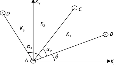
As illustrated in Figure 1, let the angle between the connection direction of well A and well B and the axis of KX be θ, let the angle between the connection direction of well A and well C AC and AB be α2, let the angle between the connection direction of well A and well D AD and AB be α3, let the permea-bility between well A and well B, well A and well C, well A and well D be K1, K2,

K3 respectively. Then, from the geometric relationship of Figure 1

1 _cos2 X _sin2 K K

m

θ

=

+ (17)

(

)

(

)

2 2 2

2 2

cos X sin

K K

m

θ α θ α

=

+ + + (18)

(

)

(

)

3 2 2

3 3

cos X sin

K K

m

θ α θ α

=

+ + + (19)

where m = KX/KY.

Assuming a2 = K1/K2, a3 = K1/K3, then formula (16)-formula (18) can get:

(

)

(

)

(

)

(

)

2 2

3 2 2 3

1 sin 1 sin

tan 2 2

1 sin 2 1 sin 2

a a

α α

θ

α α

− − −

= −

− − − (20)

(

)

(

)

2 2

1 2 2

2 2

2 2 1

cos cos

sin sin

X

Y

K K

K m

K K K

θ θ α

θ α θ

− +

= =

+ − (21)

2 2

1 cos sin

X

K =K _ θ+m θ_₍₂₂₎

Y X

[image:5.595.262.481.581.709.2]

K =K m (23) From formula (20), two angles θ1 and θ2 differing by π/2 radians can be ob-tained. Generally, the angle θ which makes m > 1 should be chosen as the angle between the AB and the KX axis, and the other angle should be the angle be-tween AB and KY. When θ is positive, rotate θ degree from AB clockwise will be the direction of KX; When θ is negative, rotate θ degree from AB clockwise

Figure 1. Schematic diagram of inter-well permeability.

K

_X

K

_Y

B

C

D

A

K

₁

K

₂

θ

α

2

α

3

(6)

will be the direction of KY, in this way, the X-Y direction in simulation grid will be determined.

In the actual reservoir simulation, due to the heterogeneity of reservoirs, grid directions within a simulation layer could be different. Generally, representative well groups can be used as basic units to calculate the directions first, and the direction of the layer and the entire simulation reservoir is obtained by weighted average [3]. In addition, grid direction which is consistent with the boundary (fault) and the direction of the flow (water injection and production well) will reduce the truncation error.

I think the method can only handle a homogeneous reservoir system. How can the heterogeneity be introduced in this method? Please add a description where you deal with multiple realizations and heterogeneity in part 2 Grid direc-tion design. What changes should be done in the mathematical formuladirec-tion (if any) to account for reservoir uncertainty and heterogeneity?

4. Case Analysis

For case analysis, please add the reference of the data source, main initial well data, and the actual well map before a schematic plot in Figure 2.

[image:6.595.207.528.480.707.2]

Well location map of Block WZ11-7-2 in WZ11-7 Oilfield in Nanhai West is shown in Figure 2, the angle (α2) between the two lines (one line is from Well WZ11-7-2 to WZ11-7-1, the other is from Well WZ11-7-2 to Well WZ11-7-4) is 30˚, the angle (α3) between the two lines ( one line is from Well WZ11-7-2 to WZ11-7-1, the other is from Well WZ11-7-2 to Well WZ11-4N-1) is 125˚. The inter-well permeability is calculated from the average log interpretation permea-bility (Table 1 into formula (20), the calculation results are θ1 = −7.7˚, θ2 = 82.3˚).

Table 1. Inter-well permeability data in Block WZ11-7-2.

Inter-well Connection Direction K K (mD)

L1 L3

WZ11-7-2 → WZ11-7-1 K1 0.045 0.1031

WZ11-7-2 → WZ11-7-4 K2 0.0588 0.1894

WZ11-7-2 → WZ11-4N-1 K3 0.0843 0.2103

Figure 2. Inter-well permeability diagram in Block WZ11-7-2.

K_X K_Y

WZ11-7-1 WZ11-7-4

WZ11-7-2

K₁ K₂

K₃

θ α2

α₃

(7)

According to formula (21): when θ1 = −7.7˚, m = 0.95 < 1; when θ1 = 82.3˚, m

= 1.2 > 1, then, θ should adopt 82.3˚. Rotating the line (WZ11-7-2 → WZ11-7-1) clockwise by 82.3˚ will obtain the X direction of L1 Formation; rotating the line

anticlockwise by 7.7˚ will obtain the Y direction. If KX adopts the value derived from geological data, KY takes 0.8 times of KX.

2) Formation L3

Similarly, a2 = K1/K2 = 0.544, a3 = K1/K3 = 0.49, according to formula (19)

θ1= −7.5˚, θ2 = 82.5˚

According to formula (21): when θ1= −7.5˚, m = 0.924 < 1; when θ1 = 82.5˚, m

= 1.43 > 1, then, θ should adopt 82.5˚. Rotating the line (WZ11-7-2 → WZ11-7-1) clockwise by 82.5˚ will obtain the X direction of L3 Formation; ro-tating the line anticlockwise by 7.5˚ will obtain the Y direction.

Based on the calculation results of the two main producing layers, rotating the line (WZ11-7-2 →WZ11-7-1) clockwise by 82.4˚ and rotating the line anticlock-wise by 7.4˚ will obtain the X and Y direction of the whole simulation area. The results are in conform with the geological analysis (the maximum principal stress orientation is 79˚ North East).

An comparison between geological analysis and the results obtained from this method is needed for verification and validation, and some kind of numerical simulation is needed to support the conclusion “which enhance the accuracy of simulation results” in Conclusion part, line 3.

5. Conclusions

1) This paper puts forward a grid direction determination method which is based on field data in reservoir simulation. In this way, the grid directions can be determined only by well location map and inter-well permeability, which en-hance the accuracy of simulation results.

2) The essence of grid direction determination is to obtain the main permea-bility direction, and the key parameter for calculating the value is inter-well permeability. Normally, the average permeability derived from well-to-well in-terference test or the log interpretation is used as the inter-well permeability.

3) While applying this method, it should be combined with geological data (such as crack direction, principal stress direction or boundary conditions), and the calculation results of this method cannot be used deliberatively.

Acknowledgements

This work is supported by the National Science and Technology Major Project of China (2016ZX05024-006).

Conflicts of Interest

(8)

References

[1] Yuan, Y.Q. and Yuan, Q.F. (1995) Application of Black Oil Model in Oilfield De-velopment. Petroleum Industry Press, Beijing.

[2] Liu, Z.R. and Xin, Q.L. (1993) Reservoir Description Principle and Method Tech-nology. Petroleum Industry Press, Beijing.

[3] Xu, W. and Gao, S.H. (1999) Grid Direction Determination in Numerical Simula-tion. Petroleum Exploration and Development, 26, 58-60.

[4] Zhang, R.J. (2004) Tensor Analysis Tutorial. Tongji University Press, Shanghai. [5] Ge, J.L. (1982) Seepage Mechanics of Oil and Gas Reservoirs. Petroleum Industry

Press, Beijing.

Nomenclature

K = Formation permeability, D

V = Seepage velocity vector, m3_/Ms

µ = Fluid viscosity, mPa·s

Φ = Fluid potential, MPa

p = Fluid pressure, MPa