GENERATION OF MAT-LAB CODE FOR ISO
AND COMPARISON WITH FINITE ELEMENT METHOD
1,*
Selendra Kumar Rajali and
1
PG student of Machine Design, NMIT, Bengaluru, India
2Department of Mechanical Engineering, NMIT, Bengaluru, India
ARTICLE INFO ABSTRACT
In this project, an attempt has been made to study and clearly explain the process between IGA FEM Method. Meshing is difficult in complex problems such as bending model where an object may move out of alignment.
investigation is carried out by both method using the same geom
observed that IGA method shows better results compare to FEM. As IGA method was quite a good method compare to FEM but it has its own disadvantage like the person needs to have a good knowledge of CAD.
Copyright © 2017, Selendra Kumar Rajali and Sunil Kumar
permits unrestricted use, distribution, and reproduction
INTRODUCTION
In this project, new method Isogeometric Method is used to analyze the partial differential equation. This
properties commonto the finite element method and some properties common with mesh-less method
Gondegaon, 2016). In FEM, the geometry of the area i separated into a set of elements.But it is challenging to separate a complexgeometry into primitive elements meshing is not an accurate creation of the geometry
2005).Meshing is the large concern in the utility of finite
elementmethod (Austin, 2005; Krishan et al.,
LITERATURE SURVEY
Sangamesh Gondegaon and Hari K. Voruganti have defined Isogeometric Analysis (IGA) wasa fresh method for uniting(CAD) and (CAE).Use of NURBS basis functions for both representation and investigation (Sangamesh
2016). J.Austin Cottrell and Thomas J.R.Hughes have studied Isogeometric analysis was impelled by the
between the (FEM) and (CAD).
*Corresponding author: Selendra Kumar Rajali PG student of Machine Design, NMIT, Bengaluru, India
ISSN: 0975-833X
Vol.
Article History: Received 17th August, 2017
Received in revised form 30th September, 2017
Accepted 29th October, 2017
Published online 30th November, 2017
Citation: Selendra Kumar Rajali and Sunil KumarH,
comparison with finite element method”, International Journal of Current Research
Key words: Spline; B-Spline, NURBS, IGA Method, FEM Method.
RESEARCH ARTICLE
LAB CODE FOR ISO-GEOMETRIC METHOD BY USING B
AND COMPARISON WITH FINITE ELEMENT METHOD
Selendra Kumar Rajali and
2Sunil KumarH, S.
PG student of Machine Design, NMIT, Bengaluru, India
Department of Mechanical Engineering, NMIT, Bengaluru, India
ABSTRACT
In this project, an attempt has been made to study and clearly explain the process between IGA FEM Method. Meshing is difficult in complex problems such as bending model where an object may move out of alignment. In this project work, both IGA and FEM flowchart is shown and a static investigation is carried out by both method using the same geometry. After, investigation it has been observed that IGA method shows better results compare to FEM. As IGA method was quite a good method compare to FEM but it has its own disadvantage like the person needs to have a good knowledge of CAD.
Kumar Rajali and Sunil Kumar. This is an open access article distributed under the Creative in any medium, provided the original work is properly cited.
In this project, new method Isogeometric Method is used to is method has many method and some less method (Sangamesh In FEM, the geometry of the area is But it is challenging to separate a complexgeometry into primitive elements. Also, accurate creation of the geometry (Austin, concern in the utility of finite
., 2013).
oruganti have defined wasa fresh method for NURBS basis functions for angamesh Gondegaon, J.Austin Cottrell and Thomas J.R.Hughes have studied sogeometric analysis was impelled by the existing gap
Selendra Kumar Rajali, PG student of Machine Design, NMIT, Bengaluru, India.
It may seem unthinkable to young engineers, but it was not long ago that computers werenowhere
offices (Austin, 2005).Vinh Phu Nguyen and St implemented that predominant technology that CAD to represent complex geometries
Rational B-spline (Vinu, Stephane
BACKGROUND
In past, before the invention of computers, numerical calculations were done by hand.Different kinds of piece function were used, among them, polynomial functions were preferred because it was easy to use
Stephane).
B-Spline
It is a type of Spline.Hughes and his co formulated a more general formulation for using B called Isogeometricmethod.
Basis Concept
B-Splines are piece-wisemathematical function defined by a rectilinear assemblage of control points.
International Journal of Current Research
Vol. 9, Issue, 11, pp.61299-61306, November, 2017
Selendra Kumar Rajali and Sunil KumarH, S. 2017. “Generation of mat-lab code for iso-geometric method by using b
International Journal of Current Research, 9, (11), 61299-61306.
GEOMETRIC METHOD BY USING B-SPLINE CURVE
AND COMPARISON WITH FINITE ELEMENT METHOD
Department of Mechanical Engineering, NMIT, Bengaluru, India
In this project, an attempt has been made to study and clearly explain the process between IGA and FEM Method. Meshing is difficult in complex problems such as bending model where an object may In this project work, both IGA and FEM flowchart is shown and a static etry. After, investigation it has been observed that IGA method shows better results compare to FEM. As IGA method was quite a good method compare to FEM but it has its own disadvantage like the person needs to have a good
Creative Commons Attribution License, which
It may seem unthinkable to young engineers, but it was not long ago that computers werenowhere to be seen in design Vinh Phu Nguyen and Stephane have predominant technology that was used by CAD to represent complex geometries was theNon-Uniform
phane).
In past, before the invention of computers, numerical calculations were done by hand.Different kinds of piece-wise function were used, among them, polynomial functions were preferred because it was easy to use (Austin, 2005; Vinu,
Hughes and his co-workers have formulated a more general formulation for using B-splines
wisemathematical function curves.It is defined by a rectilinear assemblage of basis functions and
OF CURRENT RESEARCH
Knot-Vector
It is one dimension non-decreasing knot. It divides B-Spline into a small area. This small area is known as Knot-span, which are related to elements in FEM.It is in the form
U={t1,t2,…,tn+p+1}.
Where,
p=Order of B-Spline. n=No. of Control Points.
i= Index of Knot. i.e i=1,2….,n+p+1.
Basis Function
It is determined by using Cox Recursive Formula.For, p=1
(a) Ni,p= {1 if (ti<= t< ti+1 ) or {0 otherwise.
For, p>1
(b)Ni,p=({(t-ti)/(ti+p-ti)*Ni,p-1}+{(ti+p+1 -t)/(ti+p+1 - ti+1) *
Ni+1,p-1}).
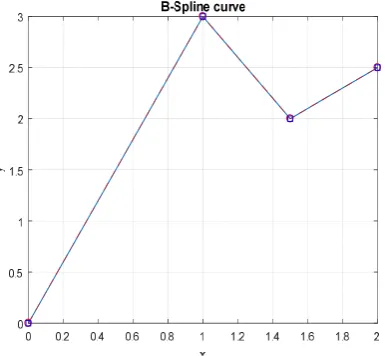
B-Spline Curve
B-Spline curvatures are defined by rectilinear assemblage of B-Spline Basis Function.B-Spline curve formula is given by;
C(t)=sum(Ni,p(t)*Bi).
Where,Ni,p(t)=Basis Function.
Bi=Control points.Z Control Points:
[image:2.595.331.541.334.512.2]X=(0 1 1.5 2);,Y=(0 3 2 2.5);
Fig. 1B-spline Curve of U={0 0 1 2 3 3}.
B-Spline Refinement
Refinement includes adding and removing of knots while meshing to solve a problem.
Knot Insertion
It is similar to formal FEM h-Refinement.In this refinement, knots are added in knot vectors, which make new knot interval or elements. e.g:U={0 0 1 2 3 3},take knot to be inserted (2).After insertion,U={0 0 1 2 2 3 3}.
Degree Elevation
It is similar to formal FEM Method p-Refinement. In this refinement, each knot value is increased by one. e.g: U={0 0 1 2 3 3}.After Elevation, U={0 0 0 1 1 2 2 3 3 3}.
k-Refinement
It is also a combined a form of Knot Insertion and Degree Elevation Refinement. e.g: U={0 0 1 2 3 3}.Insert knot (2) for Knot insertion Refinement.After Refinement,U={0 0 0 1 1 2 2 2 3 3 3}.
NURBS
B-splines are favorable for free-form representation, but they are not applied accurate representation for circle and ellipse shape.It is characterized as,
Rpi =(Ni,p *Wi)/sum(Ni,p *Wi).
Where,
R=NURBS Basis Function. Ni,p=B-Spline Basis Function. Wi=NURBS Weights Value.
Fig. 2. NURBS Basis Function of U=(0 0 0 1 2 3 3 3),p=2.
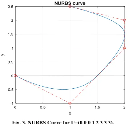
NURBS Curve
It is similar to B-Spline Curve.It is associated with control points and weights value.It is given as;
C(t)=sum(Rpi *Bi)
Where,
Rpi =NURBS Basis Function.
Bi=Control Points for B-Spline Curve.
IGA AND FEM FORMULATION
1IGA Formulation
Relevant Spaces in IGA
In IGA, physical mesh, control mesh, parameter space, and parent element are working area.
Flow Chart for IGA Method
[image:2.595.65.258.462.640.2]Start Input Data
Element Stiffness Matrix and Element load Vector.ie Ke=0,Fe=0.
Stiffness Matrix and connectivity and Connectivity
Quadrature points loop
Global Stiffness matrix Displacement Vector and Load Vector.ie K=0,F=0. NURBS/B-spline function, Derivatives for Gaussian points.
Solve KU=F Add K and F.
Assemble global stiffness, Global load vector.
[image:3.595.316.547.56.321.2]Post-processing Stop
Fig. 3. NURBS Curve for U=(0 0 0 1 2 3 3 3).
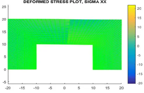
Structural Analysis for Plate with a rectangular hole
Here, for analysis, 2Dimension plate with a rectangle hole of half/symmetric portion is taken.
Input Data is given as; Young’s Modulus (E) = 1e5. Poisson’s ratio (nu) = 0.3. Load (F) = 1N.
Force load is applied on the right side and left side of the model is taken as fixed.Stress state is taken as Plane stress condition.Mat-lab code is given in Appendix A.
Geometry and Mesh
[image:3.595.57.271.183.390.2]It helps to create a model of given data using B-Spline or NURBS Curve.
Fig. 4. Model with control points.
Numerical-Integration
Element stiffness Matrix is calculated by Variational method i.e Minimum Potential Energy.
Fig. 5Knot plot of Model
Fig. 6Nrbplot of Model
K= ʃ(BTCB dpi).
Where,
K=Stiffness Matrix.
B=Strain Displacement Matrix. C=Elasticity Matrix.
Calculation of Stress
Stress is calculated by formula; Stress=C*strain.
Strain=B*U. Where,
C=Elasticity Matrix.
B=Strain Displacement Matrix. U=Displacement Value.
Solution
[image:3.595.319.541.593.767.2]The left edge of the plate is fixed.The positive load is applied on the right side of the model.
[image:3.595.58.268.610.715.2]Fig. 8Stress in the x-direction for the positive load
Flow Chart for FEM Method
Elements loop Start
Input Data
Element stiffness matrix, Load vector.ie K=0,F=0. Stiffness Matrix and connectivity
Quadrature loop
G.S.Matrix, Displacement and Load, K=0,F=0. Lagrange's function, Derivative Gaussian points Solve KU=F
Add K and F Write-Output Stop
Assemble global stiffness and load vector
Structural Analysis for Plate with a rectangular hole
Here, for analysis, 2Dimension plate with a rectangle hole of half/symmetric portion is taken.
Input Data is given as; Young’s Modulus (E)= 1e5. Poisson’s ratio (nu)= 0.3. Load (F)= 1N.
Force load is applied on the right side and left side of the module is taken as fixed.Mat-lab code is given in Appendix B.
Geometry, Mesh
In FEM meshing the element is done in different ways;
Q9 elements.
Q4 elements.
T3 elements.
Meshing is based on Gaussian Quadrature points.
Numerical-Integration
Element stiffness Matrix is calculated by Variational method i.e Minimum Potential Energy.
K= ʃ(BTCB dpi).
Where,
K=Stiffness Matrix.
Fig. 9 Geometry mesh model by Q4 element.
C=Elasticity Matrix.
Calculation of Stress
Stress is calculated by formula; Stress=C*strain.
Strain=B*U. Where,
C=Elasticity Matrix.
Solution
[image:4.595.64.264.70.234.2]The left edge of the plate is fixed.A positive load is applied on the right side of the model.
[image:4.595.311.557.364.523.2]Fig. 10 Deformed Stress for positive load
Fig. 11 Deformed Displacement in the y-direction for a positive load
Structural Analysis of a plate with a circular hole by IGA Method
[image:4.595.316.547.543.737.2]Fig. 12Control plot for given model
Fig. 13Knot plot for a model
Fig. 14Nrbplot for a model
For IGA Method
F= 1N
Fig. 15. Stress in x-direction
Fig. 16. Displacement in y-direction
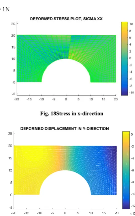
Structural Analysis for a plate with circular hole by FEM Method
[image:5.595.326.537.131.241.2]Here, for analysis, 2Dimension plate with a circular hole of half/symmetric portion is taken.
Fig. 17Geometry mesh model by Q4 element
For FEM Method
[image:5.595.316.536.288.640.2]F= 1N
Fig. 18Stress in x-direction
Fig. 19. Displacement in the y-direction
Structural Analysis of a plate with a rectangle and circular hole using Ansys
Input Data is given as; Young’s Modulus= 1e5 Poisson’s ratio=0.3 F=1N.
For Positive Load
[image:6.595.48.279.265.422.2]Fig. 20Stress for a plate with rectangle hole
Fig. 21. Stress for a plate with a circular hole
COMPARISON BETWEEN IGA AND FEM METHOD
After performing, analysis of given model by using both IGA and FEM method it is found few similarities and difference between these two methods.Some of them are discussed below;
Geometry
In IGA method, curves are used to determine area so,
it employs perfect geometry.These are not
interpolated.
In FEM method,piece-wise polynomial estimation for
the element.
Nodal points are used to define the domain of
geometry.These nodal are interpolated in Lagrange's shape Function.
Basis Function
In IGA method B-Spline/NURBS Basis Functions are
used to analysis for geometry.
In FEM Lagrange's Polynomial Basis Functions are
used to analysis for geometry.
Assembly of Global Stiffness Matrix
In IGA method, Cp-m continuity is maintained so, each
knot span shares two control points. During assembly of the matrix.
Where,p=Degree of Basis Function.
m=No. of repeated knots in the interval of knot vector.
In FEM C0 continuity is maintained at each element so, each
element shares one node during assembly of the matrix.
Meshing
In IGA method, geometry is built and the automatic
mesh is carried out.
In FEM method, meshing is carried out in a different
way;
Q9 element type.
Q4 element type.
T3 element type.
RESULT AND DISCUSSION
After performing structural analysis on a plate with rectangle hole by both method.Displacement and stress value is measured.Comparison value is listed in given table;
Table.1 for plate with rectangle hole: (Positive Load)
S.No IGA FEM ANSYS
[image:6.595.323.541.324.357.2](a). Max.Stress 21.6585 21.9709 21.7294 (b). Max.Dis. 0.0088 0.0083 0.009446
Table 2. for plate with circular hole (Positive Load)
S.No IGA FEM ANSYS
(a). Max.Stress 10.3538 10.5702 9.08378 (b). Max.Dis. 0.0043 0.0040 0.004756
In this table, IGA, FEM Method and Ansys results are calculated and analyzed for rectangle and circular hole plate.Ansys result is taken as reference for both IGA and FEM Method.It shows IGA Method result is quite closer than FEM results.
Table.3 Discretization details for a plate with rectangle hole
S.No: Properties IGA Method FEM Method (a). No.of Elements. 1792 2552 (b). No.of Nodes. 1921 2670 (c). No.of Dof. 3842 5340
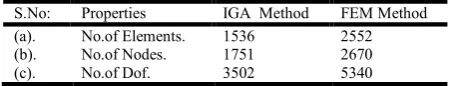
Table.4 Descretiation details for a plate with a circular hole
S.No: Properties IGA Method FEM Method (a). No.of Elements. 1536 2552 (b). No.of Nodes. 1751 2670 (c). No.of Dof. 3502 5340
It shows that for IGA Method low number of an element, nodes/control points and degree of freedom is required for the same model than FEM Method.After, investigation on both method it is concluded that for low no of elements, nodes and degree of freedom generate more accuracy with low computation compare to high no.for elements, nodes/control points and degree of freedom.
Conclusion
[image:6.595.317.548.393.426.2] [image:6.595.320.546.613.656.2]Method process.The result is compared with FEM Method on 2Dimensional elasticity problem of regular geometry by taking Ansys result as a reference.It also shows that in order to maintain the same result with IGA Method, FEM Method requires a large number of elements and control points.Due to a low number of elements and control points, IGA Method result is quite accurate than FEM Method.As, IGA method is quite fantastic than FEM, but IGA method required expertise with good knowledge of CAD.IGA Method is costly as compared to FEM.Isogeometric investigation, a new investigation method with a great deal of benefit, has a vast range in the future day.
Acknowledgement
This project was an attempt for the fulfillment of Master Degree.I would be expressed sincere gratitude and thanks to my guide Mr.Sunil Kumar H.S for completing my project.I
express gratitude to Dr. Sudhir Reeady(HOD), for
encouragement and support for this project.
Appendix.A
For IGA Method %Input Material Data.
E= ‘Input Young’s Modulus value’. nu= ‘Input Poisson’s Ratio value’. p=….% Order in u direction. q=…% Order in v direction. refineCount=….
Force(F)=Input Value.
stressState=’Plane Stress’ or ‘Plane Strain’. L=Length of the plate.
%Compute Elasticity Matrix.
C=elasticityMatrix(E0,nu0,stressState); tic; rectangleholeplate; if (refineCount) hRefinement2d end
noGps=p+1; %No of global degree of freedom. noCtrPts=noPt x*noPts y;
noDofs=noCtrPts*2;
% Compute boundary condition. bottomNodes=find(controlPts(:,2)==0)’ rightNodes=find(controlPts(:,1)==L)’; leftNodes=find(controlPts(:,1)== -L)’; topNodes=find(controlPts(:,2)==L)’; %Essential boundary condition. uFixed=zeros(size(leftNodes)); vFixed=zeros(size(leftNodes)); Plot_mesh(controlpts,weights,uKnot,vKnot,p,q,10 ‘r-’) generateIGA2DMesh. rightPoints=controlPts(rightNodes); rightEdge=zeros(noElemsV,q+1); For I=1:noElemsV rightEdgeMesh(i,:)=rightNodes(i:i+q); end
k=sparse(noDofs,noDofs); % Matrix for Global. U=zeros(noDofs,1); %Vector for displacement. F=zeros(noDofs,1);%Vector for external force aplied. % Gauss Quadrature rule.
(Wt,Q)=quadrature(nogps,’GAUSS’,2); % Loop for elements.
For e=1:noelems idu=index(e,1); idv=index(e,2); Xie=ElrangeU(idu,:); Etae=ElrangeV(idv,:); sctr=Element(e,:); SctrB=(sctr sctr+noctrlpts); n=length(sctr); D=zeros(3,2*nn); pts=controlpts(sctr,:); For gps=1:size(Wt,1) pt=Q(gps,:); wt=Wt(gps); xi=parent2ParametricSpace(xiE,pt(1)); eta=parent2ParametricSpace(etaE,pt(2)); J2=jacobianpaMapping(xiE,etaE); (dSdxi,dSdeta)=NURBS2Dders((xi;eta),p,q,uKnot,vKnot,weig hts’); jacob=pts*(dSdxi’ dSdeta’); J1=det(jacob); invJacob=inv(jacob); dSdx=(dSdxi’ dSdeta’)*invJacobi; % Compute D Matrix.
D(1,1:n)=dSdx(:,1)’; D(2,n+1:2*n)=dSdx(:,2)’; D(3,1:n)=dSdx(:,2)’; D(3,n+1:2*n)=dSdx(:,1)’; k(sctrD,sctrD)=k(sctD,sctrD)+D’*C*D*J1*J2*wt; end end Appendix.B
For FEM Method tic;
% material properties. E=Young’s Modulus. nu=Poisson’s Ratio.
stressState=’Plane Stress’ or ‘Plane Strain’; Force(F)=..input value.
% Compute elesticity matrix;
C=elasticityMatrix(E0,nu0,stressState); Rectangleplatehole.% Input data for model. % Define boundaries.
uleftn=numu*(numv-1)+1; % leftside node no of upper. urightn=numu*numv;% rightside node no.
lrightn=numu;% rightside node no.in lower. lleftn=1;%leftside node no.in lower.
rightside=(lrightn:numu:(ueftln-1); (lrightn+numu):numu:urightn)’; leftside=(urightn:-numu:(lrightn+1); (uleftn-numu):-numu:1)’; edgeelemType=’L2’; fixedXnodes=b4; fixedYnodes=b4; uFixed=zeros(length(fixedXnodes),1); vFixed=zeros(length(fixedYnodes),1); %plot mesh. Plot_mesh(node,element,ElemType,’g-’);
k=sparse(2*nnode,2*nnode);% stiffness matrix for Global. U=zeros(2*nnode,1);% Displacemenet matrix.
F=zeros(2*nnode,1);% external force matrix. xs=1:nnode;
Sctr=Element(e,:); SctrB=(Sctr Sctr+nElem); n=length(Sctr);
for q1=1:size(Wt,1) Pt=Q(q1,1); wt=Wt(q1);
(M,dMdxi)=lagrange_basis(ElemType,pt); J0=node(sctr,:)’*dMdxi;
invJ0=inv(J0); dMdx=dMdxi*invJ0; D=zeros(3,2*n); D(1,1:n)=dMdx(:,1)’; D(2,n+1)=dMdx(:,2)’; D(3,1:n)=dMdx(:,2)’; D(3,n+1:2*n)=dMdx(:,1)’;
K(SctrD,SctrD)=K(SctrD,SctrD+D’*C*D*Wt(q1)*det(J0); end
end
%Compute external force.
(Wt,Q)=quadrature(8,’GAUSS’,2); for e=1:size(rightside,1)
Sctr=rightside(e,:); Sctrx=Sctr; Sctry=Sctrx+nnode; for q1=1:size(Wt,1) pt=Q(q1,1); wt=Wt(q1);
(M,dMdxi)=lagrange_basis(EdgeelemType,pt); J0=dMdxi’*node(Sctr,:);
detJ0=norm(J0);
f(Sctrx)=f(Scytx)+M*F*detJ0*wt; End
end
Disp((num2str,(toc),’apply boundary’)) Apply BC.
U=K\f;
REFERENCES
Andrew.J.M, Michael.A.Scott, Richard, 2013. Implement B-Spline based FEM Analysis for the Boundary Value Problem, Brigham Young University, Dec.
Austin Cottrell, J., Hughes, T.J.R. 2005. IGA Integrated towards CAD and FEA, University of Texas, Austin. Brian, C. Owens, 2009. Implement of B-Spline in a
Conventional FEM Framework, Texas University, May. Hughes, T., Cottrel, J. 2005. IGA: CAD, finite element,
NURBS, exact geometry and mesh refinement, Computer method in applied mechanics and Engineering,194;4135-4195.
Kagan, A.Fischer, Yoseph,1998. New B-Spline Approach for Geometrical Design & Mechanical Analysis, International Journal for Numerical Method in Engineering.
Krishan.P.Singh, Johann.R, IGA 2013. Condition number Estimates and Fast Solver, Institute for computational and applied mathematics, May.
Sangamesh Gondegaon, Hari K. Voruganti, Static Structural and model Analysis using IGA, JTAM, Vol.46,2016,36-75. Tiller, W. 2012. Piegel, The NURBS Book, Springer.
Victor.P, Raid.S, Xuan.Z, IGA, Finite Element, University of Nice Sophia Antipolis, Department of Applied maths and Modelling, Feb,3,2012.
Vinu, Stephane.Extended Isogeometric analysis for strong and
weak discontinuities, School ofEngineeringCardiff
University, Wales, UK.