On Approximating the Gradient of the Value Function

(1)

ISSN Online: 2162-2086 ISSN Print: 2162-2078

DOI: 10.4236/tel.2019.91011 Feb. 1, 2019 126 Theoretical Economics Letters

On Approximating the Gradient of the Value

Function

Alexandre Dmitriev

1,2

1_{Department of Economics, University of Auckland, Auckland, New Zealand}

2_{Centre for Applied Macroeconomic Analysis (CAMA), Australian National University, Canberra, Australia}

Abstract

The optimality conditions for macroeconomic problems with limited com-mitment often contain partial derivatives of the optimal value function, cor-responding to the outside option. This paper contributes to the literature on recursive contracts by proposing an algorithm for approximating the gradient of the value function using simulation-based methods. Our method combines numerical solution and simulation of the model, Monte-Carlo integration and numerical differentiation. It does not suffer from the curse of dimensio-nality and is therefore convenient for models involving many state variables. The algorithm inherits the speed and accuracy limitations of the numerical solution method it relies on. Our accuracy analysis is limited to a few classical examples from macroeconomic literature.

Keywords

Dynamic Participation Constrains, Numerical Algorithm, Recursive Contracts

1. Introduction

The purpose of this paper is to propose a simple algorithm for computing partial derivatives of the optimal value function. Macroeconomic problems involving incentive compatibility constraints have received wide attention in the literature due to recent advances in dynamic optimization techniques (see [1] [2] and ref-erences therein). Often the optimality conditions for this class of problems in-volve partial derivatives with respect to endogenous state variables of the optim-al voptim-alue function corresponding to the dynamic programming formulation of an outside option. Although many numerical methods can provide an approxima-tion for the value funcapproxima-tion, there is no reason to believe that a derivative of this

How to cite this paper: Dmitriev, A. (2019) On Approximating the Gradient of the Value Function. Theoretical Economics Letters, 9, 126-138.

https://doi.org/10.4236/tel.2019.91011

Received: December 27, 2018 Accepted: January 29, 2019 Published: February 1, 2019

http://creativecommons.org/licenses/by/4.0/

(2)

DOI: 10.4236/tel.2019.91011 127 Theoretical Economics Letters

approximation will be close in any sense to the actual value of the derivative. In this note we suggest an algorithm for accurately computing these partial deriva-tives by simulation.

This issue has been previously considered in [3], in the context of a stochastic growth model with capital accumulation under one-sided lack of commitment. To circumvent the problem of finding the values of the derivatives in [3], the authors proposed a method based on the ideas of Benveniste and Scheinkman

[4]. Unfortunately, their method has limited applicability since it depends on the availability of an analytical solution for the derivatives as conditional expecta-tions of the known funcexpecta-tions of the model solution. This paper proposes a sim-ple algorithm to fill this gap in the literature.

In order to be able to use finite differences to approximate the gradient at a given point, one would need to know the values of the optimal value function at a certain set of points. Our algorithm obtains approximations of these values with arbitrary precision. Moreover, achieving this accuracy is feasible for all points in the state-space which have economic relevance.

The initial step of our algorithm involves obtaining numerical solution to a problem using a procedure which satisfies three criteria. First, it approximates some unknown function with flexible functional forms of finite elements. Second, it can deliver an accurate solution as the number of the finite elements in the function goes to infinity. Third and last, the resulting numerical solution must be such that it can be formulated as a set of policy functions approximated with flexible functional forms. The next step involves using Monte-Carlo inte-gration in order to evaluate the conditional expectation of the discounted sum of future instantaneous utilities. The final step involves applying the method of fi-nite differences to approximate the values of the partial derivatives of the value function.

The attractive features of the algorithm include its rather wide scope of appli-cability and simplicity of implementation. It can be used to study the questions of risk sharing under imperfect enforcement of contracts, as well as partnerships with limited commitment when several state variables appear in the model cor-responding to the outside option. Such models may include habit formation preferences, several types of capital, or reputational co-state variables. The sug-gested method is computationally inexpensive. It does not suffer from the curse of dimensionality and therefore it is particularly convenient for models involv-ing many state variables.

The rest of the paper is organized as follows. Section 2 discusses an example, where our algorithm proves to be useful. Section 3 sketches the idea behind the algorithm. Section 4 deals with implementation of the algorithm, while Section 5 compares it with some available alternatives. Section 6 concludes.

2. Applicability of the Algorithm: An Example

(3)

that solving it boils down to designing an optimal social contract which takes into account not only technological but also incentive and legal constraints. Our example illustrates the need for computing the gradient of the value function and its practical implementation. Furthermore, it shows that our algorithm is applicable to some widely used models, to which the method in [3] cannot be applied.

Consider a model of international risk sharing, which distinguishes itself from the canonical model [5] in two respects. First, as in [6], we introduce a friction in the credit markets. We assume that the international loans are feasible only to the extent to which they can be enforced by the threat of exclusion from partici-pation in any other international risk sharing arrangement. Second, we incorpo-rate habit formation preferences into the model. The motivation for doing this is threefold. Habits help us illustrate the features of the algorithm by expanding the set of endogenous states in the model. Habit formation preferences tend to im-prove performance of the international business cycle models [7] [8]. Finally, empirical studies suggest that habit formation is consistent with the observed consumption behavior [9]. To simplify the exposition, we assume inelastic labor supply.

The planner’s problem is to choose the sequences of consumption

{ }

cit and

investment

{ }

iit to maximize a weighted sum of utilities

{maxit it, } 0 ₁ ₀

(

,

)

I t

i it it

c i E _i λ_t β u c h

∞

= =

∑ ∑

(1)

subject to an aggregate feasibility constraint

(

)

1 1 1

, ,

I I I

it it it it

i c i i i f k

θ

= = =

+ =

∑

(2)

individual participation constraints for each i=1, ,_ I_,

(

)

(

)

0 , , , ,

j a

t it j it j i it it it

j

E ∞ β u c+ h + V k h θ

=

≥

∑

(3)

the equations of motion for the capital,

(

)

1 1 ,

it it it

k ₊ = −δ k +i (4)

the laws of motion for habits,

(

)

1 ,

it it it it

h₊ =h +λ c −h (5)

and non-negativity constraints c iit it, ≥0. We assume that productivity shocks

t

θ follow a first order stationary vector autoregressive process, and that the ini-tial values for the state variables k hi0, ,i0θi0, and the initial non-negative weights,

i

λ, are given. In addition, the usual restrictions apply to the discount factor,

( )

0,1

β∈ , the capital depreciation rate, δ∈

( )

0,1 , and the persistence of habits,

( )

0,1

λ∈ .

The outside option a

(

, ,

)

i it it it

V k h

θ

_{in the participation constraint (3)}

(4)

{ } 0

(

)

0

, 0

max ,

it it t

t it it

c i t

E β u c h

∞ =

∞

=

∑

(6)

subject to

(

,

)

,

it it it it

c + =i f k θ

(

)

(

)

1 , 1 ,

it it it it it

k ₊ = f k θ −c + −δ k

(

)

1 ,

it it it it

h₊ =h +λ c −h

with the initial values being equal to the values of the state variables k hit, ,it θit

at the moment of deviation from the optimal plan.

In addition to Equations (2)-(5), the optimal allocations, for all i s, =1, , I, must satisfy the risk sharing condition,

,

i t st

s t it

ξ

Λ = Λ where

( )

(

)

(

)

(

)

1 , 0 1 1

, 1 , 1

, 1 ,

j it j j

i t c t h

j it

a

it j i

it it j

u i t E u i t j

V _{i t} _j

h

ξ

λβ β λ

ξ µ ξ ∞ _{+ +} = + + + + 

Λ = + − _ + +

  ∂ − + +  ∂ _

∑

(7)

the intertemporal condition,

(

)

(

)

(

)

1 1

, , 1 1 1

1

, 1 a , 1 ,

it j it i

i t t i t k it it

it it it

V

E f k i t

k

ξ µ

β θ δ

ξ ξ

+ + +

+

 ∂ 

Λ = _ Λ + − − + _

∂

  (8)

the complementary slackness condition,

(

)

(

)

0

, , , 0,

j a

it t it j it j i it it it

j

E u c h V k h

µ ∞ β + + θ

=

 

− =

 



∑



and the law of motion for the co-state variables Mit+1=Mit+µit, where 1

it i Mit

ξ =λ + ₊ _, µ ≥it 0, and Mi0=0. In the equations above u i tc

( )

, denotes

(

it, it

)

it u c h

c ∂

∂ , and similar abbreviations apply to other terms1.

The gradient of the optimal value function a i

V enters the intertemporal con-dition (8) and the risk-sharing concon-dition (7). Approximation of this gradient is the purpose of the algorithm proposed in [3] and in this paper. Because both algorithms can approximate ia

(

, ,

)

it it it it

V _{k h}

k θ

∂

∂ , we will use that fact to compare

their accuracy in Section 1. Our approach can also approximate ia

(

, ,

)

it it it it

V _{k h}

h θ

∂

∂ ,

whereas [3] cannot, because the analytical solution for this partial derivative as an expectation of the known functions of the model’s solution is not available. This will be further discussed in Section 1.

(5)

3. The Algorithm

Typically, in the models with participation constraints the reservation value is the value function of the outside alternative, evaluated at the current values of the endogenous state variables, x, and exogenous shocks, s. Consider the op-timal value function at a point

(

x s,

)

as an outcome of a standard optimization problem for the outside alternative:

(

)

_{{ }} 0

(

)

0

, max , ,

t

t t t

a _t

V x s E ∞ β r x a s

=

∑

(9)

subject to

(

)

(

)

1 , , , , ,

t t t t t t t

x+ =l x a s a ∈A x s (10)

0 , 0 ,

x =x s =s

where r is an instantaneous utility function, β∈

( )

0,1 the discount factor,

{ }

st

an exogenous Markov stochastic process, xt a vector of endogenous state

va-riables, at a vector of control variables, A a feasibility correspondence and l the

law of motion for the endogenous state variables. The functional equation to this problem can be derived using the standard dynamic programming techniques. It yields a time invariant policy function f such that the optimal allocations satisfy

(

,

)

t t t

a = f x s .

The purpose of our algorithm is to find a pointwise approximation to the par-tial derivative

(

,

)

i V x s x ∂

∂ of the value function with respect to its i-th

argu-ment. The algorithm takes the following three steps:

Step I (Numerical Solution) Solve the model in (9) with a spectral method and formulate the solution in terms of approximated policy functions

(

)

ˆ ; ,

t t t

a = f

ω

x s _{, which depend on the state variables and some coefficients,}ω_.

Step II (Monte Carlo Integration) Simulate N sequences of the realizations of the stochastic process

{ }

n T₁

t t

s ₌ of size T with a starting value s0n =s, for all

1, ,

n=  N. For a each sequence

{ }

n T₀ t t

s ₌ , simulate the series of the endogenous variables

{

n, n

}

T₀

t _{t t}

x a ₌ using approximated policy functions fˆ, the equations for motion for the state variables (10), and the initial values x0n=x. Using the si-mulated series calculate the discounted sums of the instantaneous returns and average over N:

(

)

(

)

1 0

1

, N T t n, ,n n .

t t t n t

V x s r x a s

N

∑∑

= = β



Step III (Numerical Differentiation) Repeat Step II to obtain approxima-tions of the value function at two points, for instance V x

(

+ιi,s

)

and

(

_i,

)

V x−ι s , where ιi denotes a conformable vector of zeros with one on its

i-th coordinate, and  is a small positive number. Calculate the value of the partial derivative using, for example, Stirling’s finite difference formula:

(

,

)

(

,

)

(

,

)

. 2

i i

i

V x s V x s

V x s x

ι

+ − −

∂ ∂

 



(6)

The optimal choice of the method for calculating the derivatives in Step III is problem specific and its accuracy depends on the smoothness of the value func-tion. The approaches available include a variety of difference formulas, Richard-son Extrapolation, or curve fitting with cubic splines. These are described at length in the standard numerical methods texts such as [10] [11] [12].

A brief note should be made at this point on the accuracy of the algorithm. In principle, arbitrary accuracy of the approximation can be achieved, by simulta-neously increasing the dimension of the approximating family of functions in Step I, increasing the size of Monte Carlo iterations in Steps I and II, and de-creasing the denominator  in Step III. In practical applications, however, there are several sources of the approximation errors. First, in order to obtain the values of the optimal value function at a point, one relies on the approxima-tions of the policy funcapproxima-tions implied by the numerical solution to the model. Second, because we consider stochastic models, there is an additional error stemming from the evaluation of the integral in the computation of expected discounted returns. Finally, numerical differentiation introduces two more sources of error: the truncation error and the roundoff error. The truncation er-ror comes from omitting higher order terms in the Taylor series expansion. The roundoff error is associated with storing real numbers in computer’s float-ing-point format. Section 0 discusses some practical accuracy issues in the con-text of an example.

4. Implementation of the Algorithm

This section describes a practical computational strategy for implementing the algorithm using the example from Section 2. The optimality conditions include partial derivatives of the value function corresponding to the dynamic pro-gramming formulation of the agents outside option, i.e. autarky. The functional equation for the autarkic problem is:

(

)

_{( ) ( )}

{

( )

(

) (

)

}

, ,

, , max , , , | , ,

c i A k

V k h u c h E V k h k h

θ

β

θ

∈ ′ ′ ′

= + _ _

(

)

,

h′ = +h λ c h−

(

1

)

,

k′ = −δ k i+

( ) ( )

_,

{

_, 2_:

( )

_,

}

_.

A kθ = c i ∈+ c i f k+ = θ

The objective of the algorithm is to find the values of the partials Vh

( )

⋅ and

( )

k

V ⋅ at a point

(

k h, ,θ

)

_{, which is likely to happen in equilibrium. Since the}

analytical expression for these derivatives is in general unavailable, we have no choice but to rely on numerical differentiation. Another complication which arises here is that the closed form solution to the optimal value function is gen-erally unavailable too. Hence, one needs to approximate value function at two points, e.g. V k

(

+ε, ,hθ

)

_andV k

(

−ε, ,h θ

)

_{with arbitrary accuracy in order}

to be able to use the finite differencing approach.

(7)

me-DOI: 10.4236/tel.2019.91011 132 Theoretical Economics Letters

thod which can approximate the policy functions with arbitrary accuracy. This example relies on a version of stochastic simulation algorithm, which formulates the solution in terms of approximated policy functions. The Euler equation for the problem is given by:

(

)

(

)

1 1, 1 1 ,

t βEt t+ f kk t+ θt+ δ 

Λ = _Λ + − _

where marginal utility of consumption is

(

)

(

)

(

1 1

)

0

, j 1 j , .

t c t t t h t j t j

j

u c h βλE ∞ β λ u c_{+ +} h_{+ +}

=

 

Λ = + _ − _



∑



To simplify the exposition we will consider the case of non-persistent habits, which corresponds to λ=1. We assume the functional forms standard in the growth literature. The instantaneous utility function is given by

(

,

) (

)

1

t t

c bh u c h

σ

− − =

− , where b∈

( )

0,1 and σ >0. The production function

is Cobb-Douglas and is given by f k

(

t,

θ

t

)

=

θ

t tkα. The stochastic process for

productivity is logθt=ρlogθt−1+εt, where ρ∈

( )

0,1 , and

{ }

εt are

inde-pendent normally distributed random variables with zero mean and variance 2

ε

σ . In this example, we restrict attention to one particular set of the parameters which are summarized in Table 1.

The algorithm follows the three steps: 1) numerical solution; 2) Monte Carlo integration; 3) numerical differentiation.

Step I (Numerical Solution) The sequences of optimal allocations

{

c h kt, t 1, t 1

}

t ₀

∞

+ + ₌ must satisfy the following system of stochastic difference

equa-tions:

(

)

(

)

(

1

)

2 2

1 1 1 1

1 1

1

1 1 ,

t t

t t t t t

t t

c bh

c bh

E b c bh k

b c bh

σ

σ α

β αθ δ β

− − − − + + + + + + + + −    _ ₋ _      = − × + + − _{− } _     _ _ − _ _     (11)

(

)

1 1 ,

t t t t t

k

_θ

kα

_δ

k c

+ = + − − (12)

1 .

t t

h+ =c (13)

For the expositional purpose, we solve the model with a version of a stochastic simulation algorithm, which is easiest to implement (see e.g. [13]). It takes the following steps:

1) Fix the initial conditions and draw a series of

{ }

θ_{t t}T₌₁_{that obeys the law of}

motion for the exogenous shocks with T sufficiently large. To ensure sufficient accuracy of solution we chose T =50000 for all the numerical examples consi-dered. The computational burden of this is still rather low since the model needs to be solved only once.

2) Substitute the conditional expectations in (11) with the flexible functional forms that depend on the state variables k ht, ,t θt and some coefficients, ω, to

(8)

[image:8.595.209.540.90.141.2]

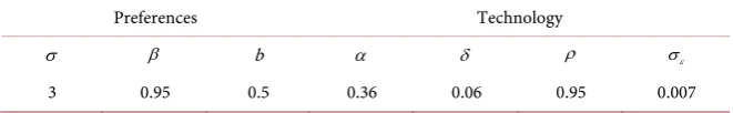
DOI: 10.4236/tel.2019.91011 133 Theoretical Economics Letters Table 1. Parameterization of the model.

Preferences Technology

σ β b α δ ρ σε

3 0.95 0.5 0.36 0.06 0.95 0.007

( )

(

ct bht

)

(

;kt

( ) ( )

,ht , t

)

,

σ

ω − ω − =βψ ω ω ω θ

where ψ ω

(

;kt

( ) ( )

ω ,ht ω θ, t

)

=exp

(

Pn

(

ω;logkt

( )

ω ,loght

( )

ω ,logθt

)

, and Pn

denotes polynomial of degree n. By using the exponent of the logarithmic poly-nomial expansion we guarantee that the left hand side of (11) remains positive. Given ct

( )

ω , the next period values for the capital and habit stocks follow

di-rectly from the laws of motion (12) and (13).

3) Using the realizations of

{ }

θ_{t t}T₌₀_{, repeat the previous step in order to obtain}

recursively a series of the endogenous variables

{

( )

, 1

( )

, 1

( )

}

₀ T

t t t _t

c ω k₊ ω h₊ ω ₌ _{, for}

this particular parameterization ω.

4) Run the following non-linear regression

( )

exp

(

;log

( )

,log

( )

,log

)

,

t n t t t t

Y ω = P ξ k ω h ω θ +η

where the role of the dependent variable Yt

( )

ω is performed by the expression

inside the conditional expectation in Equation (11).

5) Letting S

( )

ω be the result of the regression in the previous step, use an iterative procedure to find the fixed point of S, and the set of coefficients

( )

f S f

ω = ω _{. This would provide the solution for the endogenous variables}

( ) ( ) ( )

{

, 1 , 1

}

₀

T

t f t f t f _t

c

ω

k+

ω

h+

ω

₌ for this particular realization of the stochastic

process

{ }

θ_{t t}T₌₁_{along with the approximated policy functions:}

(

, ,

)

(

; , ,

)

1,

t t t t t f t t t

c k h _θ ₌bh _{+ }__{βψ ω} k h _θ _−σ



(

)

(

)

(

)

1

1 , , 1 ; , , ,

t t t t t t t t f t t t _t

k k h

_θ

kα

_δ

k bh

_{βψ ω}

k h

_θ

−σ

+ = + − − −  

(

)

(

)

1

1 , , ; , , .

t t t t t f t t t

h k h _θ bh _{βψ ω} k h _θ −σ

+ = +  

Step II (Monte Carlo Integration) Our objective is to find approximations of partials at a range of points. Supposing that the point of interest is

(

k h, ,θ

)

_the

algorithm proceeds as follows:

Simulate N sequences of the realizations of the stochastic process

{ }

n T₀ t

θ

₌ of size T with a starting value θ0n =θ , for all n=1, , N. For a each sequence

{ }

_n T₀ t

θ

₌ simulate the series of the endogenous variables

{

n, ,n n

}

T₀ t t _{t t}

k h c ₌ using

approximated policy functions, the laws of motion (12)-(13), and the corres-ponding initial values k0n=k h, 0n=h. Using the simulated series calculate the discounted sums of the instantaneous utilities and average over N,

(

)

(

)

1

1 0

1

, , .

1

n n

N T _t _t

t

n t

c bh

V k h

N

σ

θ β

σ −

= =

− −

∑∑

(9)

Step III (Numerical Differentiation) To obtain V k hk

(

, ,θ

)

get

approxima-tions of the optimal value function at V k

(

+, ,hθ

)

and V k

(

−, ,hθ

)

, where

 is a small positive number. Calculate the approximated value of the partial derivative using Stirling’s finite difference formula:

(

, ,

)

(

, ,

) (

, ,

)

. 2

V k h V k h V k h

k

θ

∂ + − −

∂

 



 (14)

The partial with respect to the habit stock is obtained in a similar way. The length of the simulated series T can be very moderate due to discounting of the future utilities. The optimal value of  is both computer and problem spe-cific.

5. Numerical Accuracy: A Comparison

This section considers the accuracy of the algorithm in the context of our exam-ple. First, we compare performance of our algorithm with the approach in [3]

when such comparison is feasible. Next, we present several special cases, which isolate the contributions of different sources to the overall approximation error.

Consider the optimality conditions for the autarkic problem, written in the sequence form:

(

,

)

(

1, 1, 1

)

(

1, 1, 1

)

,

c t t t h t t t t k t t t

u c h +βλE V k h_ ₊ ₊ θ₊ _=βE V k h_ ₊ ₊ θ₊ _ ₍₁₅₎

(

, ,

)

(

1, 1, 1

)

(

,

)

1

)

,

k t t t t k t t t k t t

V k h θ =βE V k h_ ₊ ₊ θ₊ _ f k θ + −δ ₍₁₆₎

(

, ,

)

(

,

)

(

1

)

(

1, 1, 1

)

.

h t t t h t t t h t t t

V k h θ =u c h +β −λ E V k h_ ₊ ₊ θ₊ _ ₍₁₇₎

Condition (17) can be used to compare our algorithm with the method in [3]. The latter requires solving the model numerically and expressing the derivatives of interest in terms of conditional expectations and functions of the equilibrium path of the model. Applying recursive substitution and the law of iterated ex-pectations to (17) yields:

(

)

(

)

(

)

(

)

1

, , , j 1 j , .

h t t t h t t t h t j t j

j

V k h θ u c h E ∞ β λ u c₊ h₊

=

 

= + _ − _



∑



An approximation of this derivative can be obtained by parameterizing the right hand side with flexible functional forms in the state variables

(

k ht, ,t θt

)

and running a non-linear regression using the simulated series from the numer-ical solution of the model.

Figure 1 shows the approximations of the derivative obtained using our algo-rithm and the approach in [3]. The approximated values of V k hh

(

t, ,t θt

)

are

(10)

signifi-DOI: 10.4236/tel.2019.91011 135 Theoretical Economics Letters

cantly. To see this feature, consider the range of values of capital stock in excess of 6.5. The plots of the approximate derivatives reported in the upper panel of

Figure 1 do not coincide. Moreover, the upper tail of the histogram suggests that such values of kt are not unlikely to happen in equilibrium. Notice, that while

considering a relatively high value of kt we kept the remaining arguments of

(

, ,

)

h t t t

V k h θ at their deterministic steady state values. However, the points

where capital is very high while consumption (and hence the habit stock) are at the steady state level are rather unusual. This is an expected result, since Monte Carlo integration delivers good approximations only in the region of the state space which is frequently visited by the model in equilibrium.

The framework we have chosen for a worked out example embeds several well known special cases. For instance, if λ=0, it reduces to the Brock-Mirman stochastic growth model. In this case, the analytical form of the one-period re-turn function r, which maps the graph A of the feasibility correspondence Γ into the real numbers is known. The correspondence describing the feasibility constraints is given by

(

kt,θt

)

f

(

1 δ

)

k f kt,

(

t,θt

) (

1 δ

)

kt,

Γ =_ − + − _

and the instantaneous return function becomes

(

1

)

(

) (

)

1

)

: given by t, t , t t, t 1 t t ,

r A→_ r k k₊ θ =u f k θ + −δ k k− ₊

where

{

(

)

3

(

)

}

1 1

, , : ,

t t t t t t

A= k k₊ θ ∈_₊ k₊ ∈ Γ k θ _{. Hence, by virtue of the}

Benve-niste-Scheinkman theorem the derivative of interest can be expressed as

(

,

)

(

,

) (

1

)

(

,

)

(

,

)

1 ,

k t t t t t t t k t t

V k θ =u f k′ θ + −δ k g k− θ _f k θ + −δ_

where g is the optimal policy function for capital stock. This special case allows us to compare the simulation from our algorithm with the example where the only source of approximation errors is the approximation of the policy function

g. This will allow us to isolate the contribution of the approximation errors in evaluation of the integrals and numerical differentiation to the overall approxi-mation error of the algorithm. As shown in Figure 1, the approximation deli-vered by our algorithm is very close to the approximation which relies on the Benveniste-Scheinkman theorem. Once again, in the region of the state space which is often visited by the model in equilibrium the two approximations are virtually identical. This allows us to tentatively suggest that the main contribu-tion to the approximacontribu-tion error of the algorithm comes from the approximacontribu-tion of the policy functions.

Our final special case compares the approximation of the derivative with its known exact solution. It is well known that for the functional forms

(

t, t

)

t t

f k

_θ

₌

_θ

kα_,

_{( )}

_log

t t

u c = c, and δ=1, the optimal policy function is de-fined by the simple law of motion kt+1=αβθt tkα. Moreover, the derivative of

the value function has the following analytical solution:

(

,

)

₍

₎

1 1.

1 1

t t k t t

t t t

k V k

k k

α α

αθ

α

θ

αβ

αβ θ

−

= =

(11)

[image:11.595.204.535.70.352.2]

DOI: 10.4236/tel.2019.91011 136 Theoretical Economics Letters Figure 1. Comparison with the algorithm of Marcet and Marimon [3].

By replacing the approximated policy function with the known closed form solution, we can isolate the effect of the errors stemming from Monte Carlo in-tegration and numerical differentiation on the accuracy of the approximation.

Figure 2 compares the approximated derivative obtained using the exact policy function for kt with its analytical counterpart. The reported graphs are visually

indistinguishable for the range of six standard deviations of kt around its

de-terministic steady state value. The approximation errors stemming from Monte Carlo integration and numerical differentiation are of an order of 10−9_{of the}

value of the derivative. This suggests that obtaining accurate approximation of the policy functions is crucial for the accuracy of the whole algorithm.

6. Concluding Remarks

(12)

[image:12.595.211.537.65.307.2]

DOI: 10.4236/tel.2019.91011 137 Theoretical Economics Letters Figure 2. Comparison with a Closed Form Solution.

In terms of accuracy, the algorithm demonstrates performance comparable with Marcet and Marimon’s method [3] in our benchmark example. In contrast to [3], our method is flexible enough to handle dynamic models with large numbers of state variables even when derivatives of interest cannot be expressed in terms of conditional expectations and functions of the equilibrium path of the model.

While our algorithm has wide applicability, it inherits its speed and accuracy trade-offs from the underlying numerical solution method. Our experiments suggest that obtaining accurate approximation of the policy functions is crucial for the accuracy of the whole algorithm.

An additional limitation on the algorithm’s computational speed is imposed by model’s simulation and Monte-Carlo integration. However, both steps can be parallelized along the lines proposed in [15] in order to reduce the computation-al time burden. Exploring the costs and benefits of a parcomputation-allel implementation of the algorithm is left for the future research.

Conflicts of Interest

The author declares no conflicts of interest regarding the publication of this pa-per.

References

[1] Cole, H. and Kubler, F. (2012) Recursive Contracts, Lotteries and Weakly Concave Pareto Sets. Review of Economic Dynamics, 15, 479-500.

(13)

https://doi.org/10.1016/bs.hesmac.2016.03.007

[3] Marcet, A. and Marimon, R. (1992) Communication, Commitment, and Growth.

Journal of Economic Theory, 58, 219-249.

https://doi.org/10.1016/0022-0531(92)90054-L

[4] Benveniste, L.M. and Scheinkman, J.A. (1979) On the Differentiability of the Value Function in Dynamic Models of Economics. Econometrica, 47, 727-732.

https://doi.org/10.2307/1910417

[5] Backus, D.K., Kehoe, P.J. and Kydland, F.E. (1992) International Real Business Cycles. Journal of Political Economy, 100, 745-775.

https://doi.org/10.1086/261838

[6] Kehoe, P.J. and Perri, F. (2002) International Business Cycles with Endogenous In-complete Markets. Econometrica, 70, 907-928.

https://doi.org/10.1111/1468-0262.00314

[7] Dmitriev, A. and Roberts, I. (2012) International Business Cycles with Complete Markets. Journal of Economic Dynamics and Control, 36, 862-875.

https://doi.org/10.1016/j.jedc.2011.12.006

[8] Dmitriev, A. and Krznar, I. (2012) Habit Persistence and International Comove-ments. Macroeconomic Dynamics, 16, 312-330.

https://doi.org/10.1017/S1365100510000957

[9] Chen, X. and Ludvigson, S.C. (2009) Land of Addicts? An Empirical Investigation of Habit-Based Asset Pricing Models. Journal of Applied Econometrics, 24, 1057-1093.

[10] Judd, K.L. (1998) Numerical Methods in Economics. The MIT Press, Cambridge, MA.

[11] Mathews, J.H. and Fink, K.K. (2004) Numerical Methods Using Matlab. 4th Edition, Prentice-Hall, Upper Saddle River, NJ.

[12] Press, W.H., Teukolsky, S.A., Vetterling, W.T. and Flannery, B.P. (1992) Numerical Recipes in C: The Art of Scientific Computing. 2nd Edition, Cambridge University Press, Cambridge.

[13] den Haan, W. and Marcet, A. (1990) Solving the Stochastic Growth Model by Pa-rameterizing Expectations. Journal of Business & Economic Statistics, 8, 31-34. [14] Bodenstein, M. (2008) International Asset Markets and Real Exchange Rate

Volatil-ity. Review of Economic Dynamics, 11, 688-705.

https://doi.org/10.1016/j.red.2007.12.003

[15] Creel, M. (2008) Using Parallelization to Solve a Macroeconomic Model: A Parallel Parameterized Expectations Algorithm. Computational Economics, 32, 343-352.