Bayesian Testing for Asset Volatility Persistence on
Multivariate Stochastic Volatility Models
Yong Li, Fang-Ping Peng, Hao-Feng Xu
Sun Yat-sen Business School, Sun Yat-sen University, Guangzhou, China Email: [email protected]
Received September 25, 2011; revised November 25, 2011; accepted November 30, 2011
ABSTRACT
In empirical finance, it is well-known that the volatility of asset returns is highly persistent. The persistence of the vola- tility process may be checked by testing for a unit root on stochastic volatility models. In this paper, a Bayesian test statistic based on decision theory is developed for testing a unit root on multivariate stochastic volatility models. At last, the developed approach is applied to investigate the persistent effect of financial crisis on the two main stock markets in China.
Keywords: Asset Volatility Persistency; Bayes Factor; Decision Theory; Markov Chain Monte Carlo; Unit Root
Testing; Multivariate Stochastic Volatility Models
1. Introduction
It has been well-documented in empirical literature that the volatility of asset returns is highly persistent with time, see Chou [1], Wright [2], Berger, Chaboud and Hjalmars- son [3] and Ewing and Malik [4], etc. If a persistence is observed in the log-volatility process, it means that shocks to volatility do not disappear rapidly and will remain persistent for long periods. Hence, a significant effect will be found in the security price which is caused by some changes in risk premium today. Chou [1] and Bollerslev and Engle [5] studied the volatility of the stock market and its relationship with market fluctuations. They showed that high persistence of shocks to volatility would increase the fluctuation in the volatility which caused the market to plunge. Thus, it is meaningful to develop some efficient methods to check the persistence of the shocks in the volatility process.
In empirical finance, stochastic volatility (SV) models are among the most popular models for modeling time- varying volatility clustering, so that a comprehensive un- derstanding of the types of SV models available, and the potential applications of each, is a useful foundation for research in this field. Shephard [6] provided a review of SV models and applications that was an effective base of reference.
The researchers may check the persistence of shocks in the volatility process by testing for a unit root in stochas- tic volatility models, see Wright [2]. As to the univariate SV models, So and Li [7] first developed a Bayesian unit root testing approach based on the Bayes factor (Kass and
Raftery [8]). Under Bayesian framework, the unit root test problem was regarded as a model comparison problem where two nonnested models, formulated respectively under the null and alternative hypothesis, were compared. Then, the method developed by Chib [9] was used for calculating Bayes factor. However, this method required the marginal likelihood, a marginalization over the un- known parameters and latent volatility under each model. In SV models, the number of unknown parameters and latent volatilities was very large (exceeding the number of observations), hence, obviously, the computational bur- den of the marginal likely-hood was formidable.
By introducing a weighting function rather than using Chib [9]’s method, Li and Yu [10] derived a novel form for the Bayes factor through considering the special struc- ture of the competing models. No marginalization was needed in their new form, with the result that it was more stable numerically. Further, Li, Ni and Zhang [11] pro- posed another simple numerical procedure for computing the Bayes factor to detect unit root on the basis of path sampling. This procedure was also free of complex mar- ginalization.
veloped. This continued to pose a computational chal- lenge and numerical instability. More recent literature has addressed the point-null hypothesis testing problem, for which Li and Yu [12] has developed a decisional Bayesian hypothesis testing approach to replace the Bayes factor. It was shown that the developed Bayesian test statistic may be implemented under noninformative priors, and was only a log-likelihood ratio as a by-prod- uct of Bayesian estimation, hence computationally sim- ple and stable.
As to unit root testing problem in the univariate SV models, Zhang, Li and Zhang [13] showed that the deci- sional Bayesian approach by Li and Yu [12] can achieve better finite-sample behaviors than Bayes factor. In this paper, we consider the asset return volatility persistence on multivariate SV models, which are a generalized ex- tension of univariate SV models. With the development of economic globalization, and as volatility moves to- gether across different markets, modeling volatility in a multivariate framework where the correlation structures are specified is important in many financial applications, such as international portfolio risk management, and asset allocation. The multivariate stochastic volatility setting is also important for different assets in the same financial market, because of the interwinding economic mecha- nism. More details of this issue were developed in the review paper about multivariate SV models by Asai, et al.
[14]. Also, development of the Bayesian test statistic for testing a unit root is based on the work of Li and Yu [12]. The remainder of this paper is organized as follows. In Section 2, we describe the multivariate stochastic volatil- ity models. The problem of the unit root test is discussed in Section 3. Section 4 considers an empirical application on time series data covering the subprime crisis. This paper is concluded in Section 5.
2. Multivariate Stochastic Volatility Models
The standard Multivariate SV model proposed by Harvery,
et al. [15] is given by:
1 2 1 2
1
1
, ~ 0,
diag exp 2 , ,exp 2
diag exp 2
, ~ 0, , 1, 2, ,
t t t
t pt
t
t t t t
y N
h h
h
h h N t
T
(1) where yt
p1 is the return times series,
1, 2, ,T
t t t pt
h h h h is an p-dimensional unknown log
volatility, the operator ◦ denotes the element-element product.
ut and
t
are both p-dimensional iid nor-mal error for all t. Generally, for i1, 2,,p, ,ii i
set a
s s 1.0 and is set as a diagnoal matrix.
Because the observable log-likelihood function is in- volved in intractable high-dimensional integrals, analysis of multivariate SV models is challenging. A variety of estimation methods, including simulated method of mo-ments and simulated maximum likelihood methods, have been proposed for analyzing these models. According to Yu and Meyer [16], the Bayesian method using Markov chain Monte Carlo (MCMC) techniques ranks as one of the most efficient estimation approaches. From this stand- point, we analyze the multivariate SV models of this pa- per by using MCMC techniques.
Let y
y y1, ,2 ,yT
, and 1 2 . Un- der Bayesian framework, the statistical inference is based on the posterior distribution of the parameters given the data, i.e.,
, , hT
h h h ,
p y . However, owing to the complexity
induced by latent volatility h, it is almost impossible to
evaluate the expectation of this posterior density directly. To alleviate this difficulty in the posterior analysis, we used the data-augmentation strategy (Tanner and Wong [17]) to augment the observed variable y with the latent
volatility h. Hence, instead of simulating the observations
from p
y , we generated some random observationsfrom the joint posterior distributions, i.e., p
,h y
.The simulations can be realized via a MCMC technique named Gibbs-sampler. More concretely, we start with an initial value 0, 0
h
, and then simulates one by one;
at the jth iteration, with current values j,h j :
1) Initial parameter and latent volatility h.
2) Generate j 1
h from p h
j ,y
.3) Generate j1 from
j 1,
p h y .
Observations obtained from the posterior simulation can be used for statistical inference. After the burning-in phase, that is, sufficiently many iterations of this iteration procedure, the simulated random samples can be regarded as efficient random observations from the joint posterior distribution p
,h y
.Let
j, ,j 1, 2, ,
h j J
be the simulated efficient random observations. Then, Bayesian estimates of and latent volatility h as well as their standard errors can be easily obtained via the corresponding sampling mean and sample covariance matrix. The concrete forms are given as follows:
1 1
1 1
ˆ
J J
j j
j j
J J
j j
h h
1 1
ˆ , ˆ ˆ ,
1
1 1
ˆ , ˆ ˆ ˆ .
1
T j
T j
j j
Var y
J J
h h Var h y h h
J J
3. Unit Root Testing under Decision Theory
In this paper, the persistency of volatility is equivalent to testing a root for the autoregressive coefficient on log- volatility given by:
0 1
: 1
: 1
i i
H
H
,1 (2)
As to the problem, it is known that
is the interest parameter vector, the other parameters are the nuisance parameters denoted by
1, , ,2
T p
,
.
3.1. Unit Root Testing as a Decision Problem
Generally, the observable data y in term of parameter
and parameter is fitted by some model
y ,
M p . The model
0 y 0, ,
M p denotes a model which pro-
vides a description of the probabilistic behavior of ob- servable data when the null hypothesis H0 is true. Ac-
cording to the work of Li and Yu [12], the unit root test- ing problem can be regarded as a decision problem where the action space has only two elements, namely to accept (a0) or to reject (a1) model M0 as a convenient proxy for
model M.
With regard to this decision problem, a loss function measuring the loss as a result of accepting or rejecting H0
is required to be specified. Here, we denoted this loss function as . Then, the difference
loss function denoted by
L a i, , ,i0,10
L H , ,
can be given as follows:
0, , 0, , 1, ,
L H L a L a
which measures the advantage of rejecting H0 as a func-
tion of
, . Hence, as the optimal decision, rejectingH0 will be made based on the following rule given by
0, , , d d 0
L H p y
3.2. Continuous Loss Function and Bayes Test Statistic
With regard to the hypothesis testing problem, an obvious choice is to use the Kullback-Leibler (KL) divergence func- tion as the difference loss function. However, for multivariate SV models considered in this paper, the likelihood function don’t have closed-form solution so that K-L loss function also don’t have closed-form, hence, can not be applied. Following Li and Yu [12], the continuous divergence function based on Q
mainlyused in EM algorithm is developed to replace K-L divergence function.
As to the unit root testing problem, again basing analy- sis on the work of Li and Yu [12], the continuous loss difference function can be defined as follows:
0
0 0 0
, ,
, , , ,
L H
Q Q Q Q
0
where for any 1 and 2, the Q
is given by
2
1 2 , , 1
1 2
, log , ,
log , , , , d d
h y
Q E p y h
p y h p h y h
In this situation, the Bayesian test statistic can be ex- pressed as the posterior mean of the loss function, namely,
0 0
0 0 0
, , ,
, , , ,
y
y
T y E L H
E Q Q Q Q
0
where 0 1p. As shown in Li and Yu [12], T y
,0
has an equivalent form which is given by
0
, ,
0
0 , ,
, , log
, ,
, , log
, ,
h y
y h y
p y h E
p y h
p y h
E E
p y h
(3)
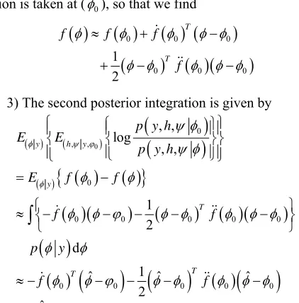
This test statistic is composed of two posterior expec- tations. The first expectation is only a by-product of a Bayesian estimation under alternative hypothesis, and is thus easily approximated using MCMC outputs. The sec- ond expectation is difficult to evaluate because it involves two simultaneous expectations, which requires tedious and time-consuming computation. Li and Yu [12] developed a convenient method for approximating this posterior inte- gration. Following their approach for the unit root testing considered here, the details of this numerical approxima- tion are simply summarized as follows:
1) Let f
logp y h
, ,
p h, y,0
d dh ,
f
f
and
2
T f
f
. It is assumed that
the regular conditions for the exchange between the inte- gration and differentiation on are satisfied, so we determine that
0 2
0
log , ,
, , d d
log , ,
, , d d
T p y h
f p h
p y h
f p h
y h
y h
sion is taken at (0), so that we find
0 0 0
0 0
1
0
2
T
T
f
f
f f
3) The second posterior integration is given by
0
0 0 0 0 0
0 0 0 0 0
, , log
, ,
1 2
d
1
ˆ ˆ ˆ
2
y h
y
T
T T
p y h
E E
p y h
E f f
f f
p y
f f
0 , ,
0
y
where ˆ is the Bayesian estimation under alternative hypothesis H1.
Remark 1: From Equation (3), it can be found that the
test statistic is the posterior expectation on the log-like- lihood ratio. Compared with the Bayes factor, which is a likelihood ratio, it is more numerically stable on compu- tation.
Remark 2: It can be proved that this test statistic can be
implemented under noninformative prior (Li and Yu [12]). Furthermore, the estimation of this test statistic is only the by-product of Bayesian estimation under null and alternative hypothesis; no additional computational ef- forts are required. This is in sharp contrast to Bayes factor.
Remark 3: In this unit root testing, a threshold value is
necessary to be used for deciding whether H0 is rejected
or not. Following the approach of Li and Yu [12], the following decision rule is used:
Accept H0 if T y
,0
C; Reject H0 if T y
,0
C where C is the threshold value. Li and Yu [12] tabulatedsome threshold values with different probability level. In this paper, we chose the critical value 3.22 as the refer- ence threshold value to express that the unit root hy- pothesis is rejected or accepted with 99% confidence. More details, one can refer to Li and Yu [12].
4. A Real Study
China stock markets are the emerging stock markets. Since their inception in 1991, they have experienced rapid de- velopments in terms of market size, trading volume, number of listed companies. For shares currently listed in China, the two stock markets—the Shanghai stock market and the Shenzhen stock market, with more than 1500 listings-conduct all trades in Chinese Yuan, The Shang- hai market accommodates the largest issuers in terms of
market capitalization and, by and large, the Shenzhen caters to small- and medium-sized concerns. In the cur- rent stage of Chinese economic development, the capital value of the Chinese stock markets positions them as one of the largest stock markets in the world, surpassed only by the stock market in the United States. Because of its growing importance, foreign investors show significant interests in the Chinese stock markets.
[image:4.595.62.273.89.303.2]On year 2007, there was a serious financial crisis. In the empirical study, we are mainly concerned whether or not the crisis had a persistent effect in Chinese stock mar- kets because of the economic globalization. The dataset of the Shanghai Composite Index (SHCI) and Shenzhen Composite Index (SZCI) over the period that covers the 2007-2008 subprime crisis was sampled. Daily closing prices for this index was collected from Yahoo.finance for the period of January 4, 2007 to April 22, 2011. The re- turn series has 1046 observations which were plotted in
Figure 1. It can be seen that the market was more vola-
tile during the period of the financial crisis.
In the case of this study, we used only the bivariate sto- chastic volatility models to fit the return series, specifi- cally, p = 2. Regarding the interest parameter , the
mixture prior is specified as follows:
1 1 1 1
~ Bernoulli(π),π~ Uniform 0,1
C
f w w f
w
,
(4)
here, to investigate the sensitivity of the prior specifica- tion, we consider three different prior distributions for
C
f , namely, Uniform(0,1) which is used to represent
prior ignorance, two informative prior distributions, Beta (10,1), Beta(20,2). As to the other nuisance parameters, some vague prior distributions are specified as follows:
1 2
2 1
~ 0.0,10 , ~ 0.0,10
~ 0.001, 0.001
N N
,(5)
Following Yu and Meyer [16], we used the WinBUGS [18] software to draw 50,000 random samples, and dis- carded the first 30,000 as burn-in samples. The conver- gence of the Gibbs sampler was diagnosed using the Raftery-Lewis diagnostic test statistic.
In Table 1, the Bayesian estimation and standard error
Figure 1. Time series plot for SHCI and SZCI returns over the period from January 4, 2007 to April 22, 2011.
Prior
Table 1. Empirical results from SHCI and SZCI index for the period covering the subprime crisis.
Statistics 1 2 1 2
2 1
2
2
Test
EST −6.937 −6.955 0.9999 66 0.9999 994 0.0038 0.0040 0.9235 0.0022 Uniform
0 0 0.
Beat1
0 0 0
Beta2
SE 0.2394 0.2041 0.0001 0.0002 0.0015 0.0010 0.0038 N/A
EST −6.884 −6.945 .999976 .999855 0.0036 0.0040 0.9246 0059
SE 0.2150 0.2583 0.0003 0.0012 0.0015 0.0016 0.0041 N/A
EST −6.829 −6.907 .999995 .999988 0.0056 0.0062 0.9249 .0023
SE 0.3078 0.2591 0.0002 0.0003 0.0020 0.0021 0.0043 N/A
at the financial sub-prime crisis happened in 2007-2008
atility models, our
prime crisis to check volatility persistence in the SHCI and
wledges the financial support of the (No.70901077), the Chi- ial Science fund (No.09YJC 790266), the Fundamental Research Funds for the Central th
had a long-lasting persistent effect in the main Chinese stock markets.
5. Conclusion and Discussions
Based on the multivariate stochastic vol
paper provides a Bayesian approach to checking persis- tence of asset return volatility. In sharp contrast to the well- known Bayes factor, the developed test statistic enjoys at least three advantages: 1) It is well-defined in noninfor- mative prior; 2) Instead of computing the likelihood ratio, it computed the logarithm likelihood ratio, so that the result is generally more stable numerically; 3) It is only a by-product of Bayesian estimation, and does not require more efforts, making its implementation simple. The ap- proach that we developed has been applied to the sub-
SZCI index return series. The empirical study confirmed that the financial crisis that happened in 2007 had some long-lasting effects in the Chinese stock markets. Noting that our test was based on the basic multivariate SV models proposed by Harvey, et al. [15], we suggest that
our technique is, itself, quite general, and can be applied in many alternative multivariate SV models (for example, factor SV models). Other possible models are discussed in Asai, et al. [14].
6. Acknowledgements
Li gratefully ackno
[image:5.595.54.541.400.521.2]Universities.
REFERENCES
[1] R. Y. Chou, “Volatility Persistence and Stock Valuation: Some Empirical Evidence Using GARCH,” Journal of Ap- plied Econometrics , pp. 279-294. doi:10.1002/ja
, Vol. 3, No. 4, 1988 e.3950030404
[2] J. Wright, “Testing a Unit Root in the Volatility of Asset Returns,” Journal of Applied Econometrics, Vol. 14, No. 3, 1999, pp. 309-318.
doi:10.1002/(SICI)1099-1255(199905/06)14:3<309::AID -JAE531>3.0.CO;2-X
[3] D. Berger, A. Chaboud and E. Hjalmarsson, “What Dri- ves Volatility Persistence in the Foreign Exchange Mar- ket,” Journal of Financial Economics, Vol. 94, No. 2, 2009, pp. 192-213. doi:10.1016/j.jfineco.2008.10.006 [4] B. T. Ewing and F. Malik, “Estimating Volatility Persis-
tence in Oil Prices under Structural Breaks,” The Finan- cial Review, Vol. 45, No. 4, 2010, pp. 1011-1023.
doi:10.1111/j.1540-6288.2010.00283.x
[5] T. Bollerslev and R. F. Engle, “Common Persistence in Conditional Variance,” Econometrica, Vol. 61, No. 1, 1993, pp. 167-186. doi:10.2307/2951782
[6] N. Shephard, “Stochastic Volatility: Selected Reading,”
ournal of Business and Oxford University Press, Oxford, 2005.
[7] M. K. P. So and W. K. Li, “Bayesian Unit-Root Testing in Stochastic Volatility Models,” J
Economic Statistics, Vol. 17, No. 4, 1999, pp. 491-496. doi:10.2307/1392407
[8] R. E. Kass and A. E. Raftery, “Bayes Factor,” Journal of the Americana Statistical Association, Vol. 90, No. 430, 1995, pp. 773-795. doi:10.2307/2291091
[9] S. Chib, “Marginal Likelihood from the Gibbs Output,” Journal of the American Statistical Association, Vol. 90,
No. 432, 1995, pp. 1313-1321. doi:10.2307/2291521 [10] Y. Li and J. Yu, “A New Bayesian Unit Root Test in
Stochastic Volatility Models,” Research Collection School
an Unit Root Testing in of Economics, Paper 1240, 2010.
[11] Y. Li, Z. X. Ni and J. Zhang, “An Efficient Stochastic Simulation Algorithm for Bayesi
Stochastic Volatility Models,” Computational Economics, Vol. 37, No. 3, 2011, pp. 237-248.
doi:10.1007/s10614-011-9252-4
[12] Y. Li and J. Yu, “Bayesian Hypothesis T
Variable Models,” Journal of Econometrics, Vol. 166, No. esting in Latent 2, 2012, pp. 237-246.doi:10.1016/j.jeconom.2011.09.040 [13] J. Zhang, Y. Li and J. Zhang, “Bayesian Testing a Unit
Root in the Volatility of Asset Returns: An Empirical
ometric Review, Vol. Comparison,” Working Paper, 2011.
[14] M. Asai, M. AcAleer and J. Yu, “Multivariate Stochastic Volatility Models: A Review,” Econ
25, No. 2-3, 2006, pp. 145-175. doi:10.1080/07474930600713564
[15] A. C. Harvey, E. Ruiz and E. Shephard, “Multiva chastic Variance Models,” Review of
riate Sto- Economic Studies, Vol. 61, No. 2, 1994, pp. 247-264.
doi:10.2307/2297980 [16] J. Yu and R. Meyer, “Multi
Models: Bayesian Estimation and Model Comparison,” variate Stochastic Volatility Econometric Review, Vol. 25, No. 2-3, 2006, pp. 361-384.
doi:10.1080/07474930600713465
[17] T. A. Tanner and W. H. Wong, “The Calculation of Pos terior Distributions by Data Aug
- mentation,” Journal of the American Statistical Association, Vol. 82, No. 398, 1987, pp. 528-549. doi:10.2307/2289457
Appendix: Calculation of
T y
,
0
for
Multivariate Stochastic Volatility Model
As to the multivariate stochastic volatility model con-
sidered in this paper, the joint density function for the observable data and latent volatility is given by:
1 11 1 1 1 1 1 1 1 1 1 , , , , , , , , ,
, , , , exp
2
exp
2
T
t t t t
T T
t t t t
t t t t
t t
T
t t t t
t
p y h p y h h
y y
p y h p h h C
h h h h
where C is a known constant. The observable likelihood
function can be expressed as:
,
dp y
p y h hHere, it can be seen that owing to the latent volatility, the
observable likelihood function is a high-dimensional mul- tiple integral which does not the closed-from expression.
According to Section 3, to approximate the Bayesian test statistic, T y
,0
, several components are derived as follows:
0
0 0
log , , , , log , , , , log , , , , log , ,
log , , , , log , , log , , , , log , , , ,
p y h p y h p y h p
p y h p p y h p y h
0
As to the bivariate multivariate SV model in this empirical study, we may derive the concrete form given by:
0 2 2 20,1 1 1, 1 1 0,1 1 1 1 1, 1 1 2
1 ,11
2 2 2
0,2 2 2, 1 2 0,2 2 2 2 2, 1 2 2
1 ,22
log , , , , log , , , , 1 2 2 1 2 2 T
t t t
t T
t t
t
p y h p y h
h h h
h h
h t Moreover,
0 0 1 0 11 1 1 1, 1 1 1, 1 1 , , ,
1 ,11 2
1 2 0 , , ,
,11 1
log , , , ,
, , , , d d d d
1
,
log , , , , 1
, , , , d d d d
T
t t t
h y
t
h
p y h
f p h y h
E h h h
p y h
f p h y h E
h
0 2 1, 1 1 11
2 0
2
2 2 2 2, 1 2 2, 1 2 , , , 1 ,22 2 2 2 2 , 0.
log , , , ,
, , , , d d d d
1
,
log , , , ,
, , , ,
T t t
T
t t t
h y
t
f
p y h
f p h y h
E h h h
p y h
f p h y
0 20 , , , 2
1 ,22 2
1
d d d ,
0.
T t h
t
h d E h
f
, 1 2