1. Determine the impulse responses for the following systems: a) 2( t

ECE 300

Signals and Systems Homework 4

Due Date: Thursday April 2, 2009 at the beginning of class Exam 1, Monday April 6

Problems

1. Determine the impulse responses for the following systems:

a) 2( )

( ) ( ) ( )

t t

y t x t e− −λ x λ λd −∞

= +

∫

1 ( )

( ) ( 2)

t t

y t e λ x λ dλ −

− −

−∞

=

∫

c) 2 (y t )−y t( )=3 (x t+2) d) ( ) 1 ( )

t

t I

y t x d

I ₋ λ λ

=

_∫

2. Consider the following two subsystems, connected together to form a single LTI system.

Determine the impulse response of the entire system if the impulse responses of the subsystems are given as:

( ) h t

a) 1( ) ( ) 2( ) 2 ( )

t

h t =δ t h t = e u t−

b) 1( ) ( ) 2( ) 2 ( 1)

t

h t =e u t− h t = δ t−

−

t u t

c) ( 1) ( 1)

1( ) ( 1) 2( ) ( 1)

t t

t e u t h t e u

h = − + + = − − t

d)h₁( )t =u t( )−u t( −1) h₂( )= ( )

Use analytical convolution when evaluating the convolution integrals in this problem.

1( )

h t h t₂( )

( ) v t( )

3. Consider a causal linear time invariant system with impulse response given by ( 1)

( ) t ( 1)

h t =e− − u t−

The input to the system is given by

( ) ( ) ( 1) ( 3)

x t =u t −u t− +u t−

Using graphical convolution, determine the outputy t( ) for 2≤ ≤t 5. Note the limited range of t we are interested in !

Specifically, you must

a) Flip and slideh t( )

b) Show graphs displaying both h t( −λ) and x( )λ for each region of interest c) Determine the range of t for which each part of your solution is valid d) Set up any necessary integrals to compute y t( )

e) Evaluate the integrals

You should get (in unsimplified form)

( 1) 1

( 1) 1 ( 1) 1 3

[ 1] 2

( )

[ 1] [ ] 4

t

t t t

e e t

y t

e e e e e t

− −

− − − − −

⎧ 4

5

− ≤ ≤

= ⎨

− + − ≤

⎩ ≤

4. Consider a causal linear time invariant system with impulse response given by ( 1)

( ) t ( 1)

h t =e− − u t−

a) Show that the step response of the system (the response to a unit step) is ( 1)

( ) [1 t ] ( 1)

s t e u t

y = − − − −

b) Using linearity and time-invariance, determine the response of the system to the input

( ) ( 1) 2 ( 2)

x t =u t− − u t−

c) Use graphical convolution to determine the output of the system. d) Show that your answers to b and c are the same.

5. Consider a causal linear time invariant system with impulse response

2

( ) 1 0.5 [ ( 2) ( 1)]

h t = −⎡_⎣ t ⎤_⎦ u t+ −u t−

The input to the system is

( ) ( 1) ( 1) 2 ( 2) 2 ( 3)

x t =u t+ −u t− − u t− + u t−

These two functions are plotted below:

-4 -3 -2 -1 0 1 2

-1.5 -1 -0.5 0 0.5 1 1.5

Time (sec)

h(t

)

-2 -1 0 1 2 3 4

-2 -1 0 1

Time (sec)

x(

t)

Using graphical convolution, set up the integrals to determine the outputy t( )

Specifically, you must

• Flip and slide h t( )

• Show graphs displaying h t( −λ) relative to x( )λ for each region of interest.

• Determine the ranges of for which each part of your solution is valid. t

• Set up any necessary integrals to compute . Your integrals must be complete and simplified as much as possible (no unit step functions)

( ) y t

6. (Matlab/Prelab Problem, read the Appendix for help) From the class website download the files homework4.m and convolution.m. homework4.m is a script file that sets up the time arrays and functions, and the invokes the function

convolution.m to compute the convolution of the two functions. Homework4.m then plots the two functions to be convolved, and then the resulting convolution of the two functions.

a) Complete the code for the function convolution.m.

b) Use the script homework4.m to compute and plot the convolution of the functions ₁( )

2 t x t =rect⎛ ⎞_{⎜ ⎟}

⎝ ⎠ and 2

1 ( )

3 t x t =rect⎛_⎜ −

⎝ ⎠

⎞

⎟. If you have done this correctly,

you results should like those shown in Figure 1. Turn in your plot.

c) Use the script homework4.m to compute and plot the convolution of the functions 1

2 (

2

) t

t re t

x = c ⎛_⎜ − ⎞

⎝ ⎠⎟ and 2

2.5 5

( ) t

x t =rect⎛_⎜ −

⎝ ⎠

⎞

⎟.If you have done this

correctly, you results should like those shown in Figure 2. Turn in your plot.

d) For the remainder of this problem, assume we want t1 to go from -1 to 6 with an increment of 0.01 and t2 to go from -1 to 8 with an increment of 0.01. Then find the convolution of each of the following:

1 2

1 2

1 2

2.5

( ) rect ( ) ( )

5

1

( ) rect ( ) ( )

2

0.1

( ) rect ( ) ( )

0.2

t

t

t

t

x t x t

t

e u t

x t x t

t

e u t

x t x t

− − − − ⎛ ⎞ = _{⎜ ⎟} = ⎝ ⎠ − ⎛ ⎞ = _{⎜ ⎟} = ⎝ ⎠ − ⎛ ⎞ = _{⎜ ⎟} =

⎝ ⎠ e u t

Turn in your plots and your code. Note: In this part we can view this as looking at the response of a system with impulse response to inputs which are pulses of decreasing width. This is what we will be doing in Lab 3 when we try to model an impulse,

( ) t ( ) h t =e u t−

( )t

-2 -1.5 -1 -0.5 0 0.5 1 1.5 2 0

0.2 0.4 0.6 0.8 1

x1

(t

)

-2 -1 0 1 2 3 4

0 0.2 0.4 0.6 0.8 1

x2

(t

)

-4 -3 -2 -1 0 1 2 3 4 5 0

0.5 1 1.5 2

Time (sec)

y(

t)

Figure 1: Results for problem 6-b

Figure 2: Results for Problem 6-c.

-1 -0.5 0 0.5 1 1.5 2 2.5 3 3.5 4 0

0.2 0.4 0.6 0.8 1

x1

(t

)

-2 -1 0 1 2 3 4 5 6 7 8 0

0.2 0.4 0.6 0.8 1

x2

(t

)

-2 0 2 4 6 8 10 12

0 0.5 1 1.5 2

Time (sec)

y(

7. Pre-Lab Exercises (to be done by all students. Turn this in with your homework and bring a copy of this with you to lab!)

a) Calculate the impulse response of the RC lowpass filter shown in Figure 1, in terms of unspecified components R and C. Determine the time constant for the circuit.

+

C1

Vout

-+

0

+

-V1

+ R1

Figure 1. Simple RC lowpass filter circuit.

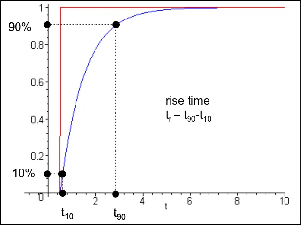
b) Show that the step response of the circuit (the response of the system when the input is a unit step) is , and determine the 10-90% rise time. , as shown below in Figure 2. The rise time is simply the amount of time necessary for the output to rise from 10% to 90% of its final value. Specifically, show that the rise time is given by

/

( ) (1 t ) ( )

s t e u

y = − − τ

ln(9)

r

t

t

r

t

τ =

t₉₀

t₁₀

rise time

tr= t90-t10

90%

10%

t₉₀

t₁₀

rise time

tr= t90-t10

90%

10%

c) Specify values R and C which will produce a time constant of approximately 1 msec. Be sure to consider the fact that the capacitor will be asked to charge and discharge quickly in these measurements.

d) Using linearity and time-invariance, show that the response of the circuit to a pulse of length T and amplitude A (, i.e. a pulse of amplitude A starting at 0 and ending at T) is given by

/ ( )/

( ) (1 t ) ( ) (1 t T ) ( )

pulse

y t =A −e− τ u t −A −e− − τ u t T−

e) Assume the input is a pulse of amplitude A and width T, and use the results from part d to determine an expression for the amplitude of the output at the end

of the pulse, y_pulse( )T . Next, assume that T 1

τ (the duration for the pulse is

much small than the time constant of the circuit) and use Taylor series

approximations for the exponentials to show thaty_pulse( )T AT τ

≈ . This means the

Appendix

Although this is a continuous time course, and Matlab works in discrete-time, we can use Matlab to numerically do convolutions, under certain restrictions. The most important restriction is that the spaces between the time samples be the same for both functions. Another other restriction is that the functions really need to return to zero (or very close to zero) within the time frame we are examining them. Finally, we need fine enough resolution (the sampling interval must be sufficiently small) so that our sampled signals are a good approximation to the continuous signal. We will discuss sampling at the end of the course.

First, we need to have two functions to convolve. Let’s assume we want to

convolve the functions 1( )

2 t x t =rect⎛ ⎞_{⎜ ⎟}

⎝ ⎠ and 2

1 ( )

3 t x t =rect⎛_⎜ − ⎞_⎟

⎝ ⎠.

Let’s denote the time vector that goes with x₁ as t1, and the time vector that goes with x₂as t2. Then we create the functions with something like

t1 = [-3:0.01:3]; t2 = [-2:0.01:4];

x1 = @(t) 0*(t<-1)+1*((t>=-1)&(t<=1))+0*(t>1);

x2 = @(t) 0*(t<-0.5)+1*((t>=-0.5)&(t<=2.5))+0*(t>2.5);

Next we will need to determine the time interval between samples. We can determine this as

dt = t1(2)-t1(1);

It doesn’t matter if we use t2 or t1, since the sample interval must be the same.

Now we can use Matlabs conv function to do the convolution. However, since we are trying to do continuous time convolution we need to do some scaling. To understand why, let’s look again at convolution:

( ) ( ) ( )

y t x λ h t λ λd ∞

−∞

=

∫

If we were to try and approximate this integral using discrete-time samples, with sampling interval Δt, we could write

( ) ( )

( ) ( )

( ) ([ ]

y t y k t x x n t h t h k n t

λ

λ )

≈ Δ

≈ Δ

We can then approximate the integral as

)

( ) ( ) ( ) ( ) ( ) ([ ] ) ( ) ([ ]

n n

n n

y t x λ h t λ λd y k t x n t h k n t t t x n t h k n

∞ =∞ =∞

=−∞ =−∞

−∞

=

_∫

∑

∑

( ) ([ ] )

n

n

t

The Matlab function conv computes the sum x n t h k n t

=∞

=−∞

Δ − Δ

∑

t , so to

approximate the continuous time integral we need to multiply (or scale) by Δ . Hence

y = dt*conv(x1,x2);

Finally, we need to determine a time vector that corresponds to y. To do this we need to determine where the starting point should be. Let’s consider the convolution

( ) ( ) ( )

y t x λ h t λ λd ∞

−∞

=

∫

Let’s assume x t( ) is zero until time , so we could write t1 x t( )=x t u t( ) ( −t1) for some functionx t( )

( ) h t h

. Similarly, let’s assume is zero until time , so we

could write for some function . The convolution integral is then

( )

h t t2

2 ( ) (t u t t )

= − h t( )

2

1

1 2

( ) ( ) ( ) ( ) ( ) ( ) ( )

t t

t

y t x λ λu t h t λ u t λ t dλ x λ h t λ d −

∞

−∞

=

∫

∫

This integral will be zero unless t− ≥t1 t2, or . Hence we know that is zero until . This means for our convolution, the initial time of the output is the sum of the initial times:

1 t≥ +t t2

( )

y t + t=t1 t2

initial_time = t1(1)+t2(1);

Every sample in y is separated by time interval dt. We need to determine how long y is, and create an indexed array of this length

n = [0:length(y)-1];

Finally we can construct the correct time vector (ty) that starts at the correct initial time and runs the correct length