Rule Based Classification System for Medical Data Mining Using Fuzzy Ant Colony Optimization

(1)

Rule Based Classification System for Medical

Data Mining Using Fuzzy Ant Colony Optimization

Mostafa Fathi Ganji, Mohamad Saniee Abadeh

Mostafa Fathi Ganji is with Faculty of Electrical and Computer Engineer-ing, Tarbiat Modares University, Nasr Bridge, Jalal Ale Ahmad Highway, TEHRAN, IRAN (email: m.ganji@modares.ac.ir)

(2)

2. ANT COLONY OPTIMIZATION (ACO)

Ant algorithms are based on the cooperative behavior of real ant colonies, which are able to find the shortest path from a food source to their nest [2]. While walking, real ants deposit a chemical substance called pheromone on the ground. Ants can smell pheromone and when choosing their way, they tend to choose, in a probabilistic way, paths marked by strong pheromone concentrations [19]. In the absence of pheromone, ants choose paths randomly. Pheromone is evaporated over time, therefore, in shorter paths pheromone evaporation is less in comparison with longer paths and causes more pheromone accumulation in the shorter routes [15]. This positive feedback effect means that because of more pheromone all the ants will eventually use the shortest path [16]. Although a single ant is capable of building a solution (i.e., a path), the optimal solution comes about solely as a result of the cooperative behavior of the ant colony (which is based on a simple form of indirect communication through the pheromone, called stigmergy). Although the first ACO algorithm, called Ant System, was applied to solve the TSP problem [7], a large number of applications to other problems were proposed after the introduction of ant system. Recently, the ACO metaheuristic was proposed as a common framework for existing applications [19]. Each ant builds a possible solution to the problem by moving through a finite sequence of neighbor states (nodes). Moves are selected by applying a stochastic local search directed by the ant internal state, problem-specific local information and the shared information about the pheromone [2].

3. PROPOSED METHOD

FC-ANTMINER operates in two main stages: Training Stage and Testing Stage. In training stage, at first, the ACO algorithm is applied to generate a set of fuzzy rules via training patterns. These fuzzy rules are displayed as the following form:

Rule Rj:

If x1 is Aj,1 and … and xn is Aj,n , then Class Cj with CF=CFj.

Where Rj is the label of the jth fuzzy if–then rule, Aj1,…, Ajn are antecedent fuzzy sets on the unit interval [0,1] (each triple <attribute, operator, value> called a term), Cj is the consequent class (i.e., one of the given c classes), and CFj is the grade of certainty of the fuzzy If–then rule Rj. The antecedents of each fuzzy rule are presented in the form of typical set of linguistic values as figure 1. The membership function of each linguistic value in figure 1 is specified by homogeneously partitioning the domain of each attribute into symmetric triangular fuzzy sets. We use such a simple specification in computer simulations to show the high performance of our fuzzy classification system, even if the membership function of each antecedent fuzzy set is not tailored. However, we can use any tailored membership functions in our fuzzy classifier system for a particular pattern classification problem.

ACO learns the rules associated to each class separately. Therefore, if we have c classes then we will have c rule sets, each one corresponding to its related class. All these rule sets make our final classification system. Figure 2 shows the training stage of Fc-AntMiner.

3.1 Fuzzy Rule Generation by ACO

[image:2.595.388.503.105.261.2]

The ACO algorithm applies the artificial ants to explore among the training patterns and gradually deriving fuzzy rules. The ants learns the rules related to each class separately, that is, for each

Figure 1. The used antecedent fuzzy sets in this paper. a) 1: Small, 2: medium small, 3: medium, 4: medium large, 5: large. b) 0: don’t care.

Figure 2. The ACO algorithm is applied to generate a set of fuzzy rules related to each class separately, via training samples.

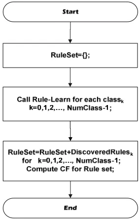
class such as k a function is called to learn the corresponding fuzzy rules. Figure 3 shows the stages of fuzzy rule generation by ACO. At first, the output rule set is empty and to learn the fuzzy rules associated with each class, Rule-Learner function (figure 4) is called. This function learns the fuzzy rules corresponding to each class and returns them to main learning algorithm. All of the learned rules for each class could be used as our final classification system.

In Rule-Learner function (figure 4), the list of discovered rules is empty and the training set consists of all the training cases. In outer loop of Rule-Learn, the pheromone is initialized in a way that all cells in the pheromone table are initialized according to equation (1) [4]:

Then, the first ant (ant0) constructs rule Rj randomly by adding one term (each triple <attribute, operator, value> called a term) at a time and in the next iterations (t≥1) the ants modify rule Rj. The maximum terms that each ant can modify in each iteration (t≥1) is

S MS M ML L

Membership

a) Attribute Value

0.0 1.0

1.0

Membership

b) Attribute Value 0.0

1.0

1.0 DC

Training Stage

τ,t 0 _∑

[image:2.595.303.548.294.491.2]

(3)

[image:3.595.98.240.115.338.2]

Figure 3. The stages of fuzzy rule learning by ACO

1- J=0;

2- TrainingPatterns= {all training samples}; 3- DiscoverdRulesk= {};

4- Repeat

4.1- t=0, Set Pheromone Table; 4.2-Update Heuristic matrix (Hk); 4.3- Antt makes Rule Rj; 4.4- While (t<Max_ants)

4.4.1- Antt modifies Rj;

4.4.2- Computing the quality of Rj; 4.4.3- Updating the pheromone; 4.4.4- t++;

4.5-The ant that has the best modification augments its rule to DiscoverdRulesk;

4.6- Remove the cases correctly covered by the selected rule from the TrainingPatterns;

4.7- J++;

5- Until (Stopping Conditions are satisfied) 6- Return DiscoverdRulesk;

7- End.

Figure 4. Rule_Learner Function.

determined by a parameter named Max_change. Max_change can be the number of attributes at most.

Each ant chooses termi,j to modify (or add to current rule in the first iteration) with following probability:

Where, ηi,j is a problem-dependent heuristic value for termij. The function that defines the problem-dependent heuristic value will be discussed in section (3.1.1)

τi,j is the amount of pheromone currently available(at time t) on the path between attribute i and value j.

a and bi are the total numbers of values in the domain of attributei and is the total number of attributes respectively. I is the set of attributes that are not yet used by the ant

The number of ants that modify the rule Rj in inner loop of FC-AntMiner is determined by user-defined parameter, named Max_ants.

While a rule modified by an ant, the quality function calculates the quality of modified rule. The quality of a rule such as Rj is computed according to equation (5) [13].

f

∑_| µ

∑_| 3

f

∑| _!w µ x

∑| _!w 4

Q = wpfp – wnfn (5) Where

FP: rate of positive training samples covered by the rule Ri. FN: rate of negative training samples covered by the rule Ri Wk: a weight which reflects the frequency of instance xk in the training set.

WP: the weight of positive classification. WN: the weight of negative classification.

After each ant modifies the terms of a rule according to Max-change parameter, pheromone updating is carried out. We have defined a new simple method to update pheromone, in a way that whenever each ant modified the terms of rule Rj, quality of rule Rj is calculated. If the quality of rule Rj is increased then pheromone of this rule is increased according to value of quality that has been improved. Our experiments have shown that by this new update strategy, in each iteration, the pheromone helps the ants to improve the quality of rule effectively. Pheromone updating is carried out according to equation (7).

∆Q =QiAfter Modification – QiBefor Modification (6)

Where

∆Q shows difference between the quality of the rule Ri after and before modification. C is a parameter to regulate influence of improved quality to increase the pheromone (in our experiment C is 0.5).

It is necessary to decrease the pheromone of terms that have not participated in the construction of rules. For this purpose, pheromone evaporation is simulated. To simulate the pheromone evaporation in real ant colony, the amount of pheromone associated with each termij that does not occur in the constructed rule must be decreased.The pheromone of unused terms is decreased by dividing the amount of the value of each τij by the summation of all τij [4].

Stopping condition in outer loop of Rule-Learner (figure 4) function refers to any condition that user has defined to terminate the loop. In our experiments, when minimum uncovered instances

$%,&

'_%,&( .*%,&

∑ ∑ '/% .%& %,&( .*%,& ,+%,- 2

(4)

are remained or fairly all ants travel in the same path, the learning process is finished.

For each class independently, the above operations will be done iteratively and finally a set of rules would be discovered. These rules could be used as our classifier.

3.1.1 Heuristic Information

[image:4.595.65.271.313.402.2]

The ants modify the terms of the rules according to heuristic information and amount of pheromone. Fc-AntMiner has used a set of two-dimensional matrixes, named H, as heuristic information so that H= {H1, H2, …, HnumClass}. For each class such as k we have matrix Hk which rows and columns indicate the attributes and fuzzy values respectively. Hk shows the distribution of the values of data set in class k. Each time a rule is discovered and correctly covered patterns are removed, set H is updated and it won't be changed in the inner loop of Rule-Learn function. Therefore, the computation overhead to calculate the heuristic information is significantly reduced. Also these matrixes help the ants to choose more relevant terms and make strong rules. Each member of set H such as Hk is represented as follow:

Fig.5.Matrix Hk shows the distribution of data set values (class k) An entry of matrix Hk such as hi,j (j>1) shows the number of uncovered patterns that labelled with class k and value of attributei is equal to jth fuzzy value, j=1,2,...,6 (DC is 1th fuzzy value, S is 2th fuzzy value, …).

First column (hi,1 i=1,2,..,n) includes the don't care (DC) probability of features. Saniee et al [14] used a constant value to determine DC probability of the features value which was calculated with trial and error. FC-ANTMINER to determine the don’t care value of each attribute such as attributei uses the uniformity measurement of domain values of attributei. The lesser value of DC shows the more uniformity distribution of the attribute values are and vice versa. So, if DC value of attributei is equal to 1 and 0, it means that the domain values of attributei have completely uniform distribution and none-uniform distribution respectively. For each attribute, DC value is measured in terms of the entropy. Therefore, the first column of matrixes in set H is updated by the following equations:

hi,1=1-Ei,1 (9)

Where

sumhi is the summation of none-DC values of attributei and p (hi,j|sumhi) is the empirical probability of observing the hi,j.

It is essential to normalize the entries of matrixes set H to facilitate its use in Equation (5). The following normalization

function has been applied to normalize the matrixes entry:

Where Max2h_,6 is maximum value in column j and η, is heuristic information (this value is used in equation (5)).

3.2 Fuzzy Inference

Let us assume that our pattern classification problem is a c-class problem in the n-dimensional pattern space with continuous attributes. We also assume that M real vectors xp= (xp1, xp2, …, xpn), p=1,2, …, m are given as training patterns from the c classes (c<<M).

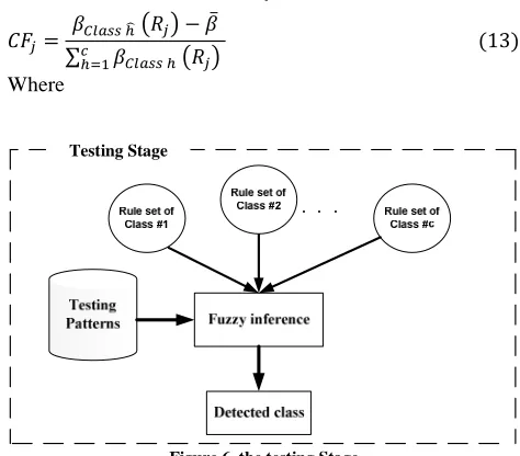
When ACO-learning algorithm, corresponding to each class, generated a set of fuzzy rules using M patterns, a fuzzy inference engine is needed to classify test patterns (figure 6). For this purpose, certainty grade must be computed. The following steps are applied to calculate the certainty grade of each fuzzy if-then rule: [6]

Step 1: Calculate the compatibility of each training pattern xp= (xp1, xp2, …, xpn) with the fuzzy if–then rule Rj by the following product operation:

<=2>?6 <=2>?6 @ … <=B2>?C6,D 1,2,3, … , E 11

Where <_=F2>_?F6 is the membership function of ith attribute of pth pattern and M denotes the total number of patterns.

Step 2: For each class, calculate the relative sum of compatibility grades of the training patterns with the fuzzy if–then rule Rj:

GHIJKKL2M=6 N _O<=2>?6 HIJKKL PQRHIJKKL

, S 1,2, … , T 12

Where G_HIJKKL2M₌6 is the sum of the compatibility grades of the training patterns in Classh with the fuzzy if–then rule Rj and

OHIJKKL is the number of training patterns which their corresponding class is i.

Step 3: The grade of certainty CFj is determined as follows [13]:

UV=_∑GHIJKK LW_G 2M=6 X GY HIJKK L 2M=6 Z

L[ 13 Where

Figure 6. the testing Stage

DC S MS M ML L

\

Att1

Att2

Attn-1

]

^

_

S1,1 S1,2 S1,3 S1,4 S1,5 S1,6

S_2,1

\

SbX1,1

c

\

Sb,1 Sb,2 Sb,3 Sb,4 Sb,5 Sb,6

d

e

f

E, X N P2h,isumh6 m

[n

. logP2h,isumh6 , i 1,2, … , n 8

η_, h,

Max2h,6, + i 1,2,3, … , n 10

Hk=

[image:4.595.306.543.493.701.2]

(5)

GY ∑L!Lvu_{T X 1}GHIJKK L 2M=6 14

Now, we can specify the certainty grade for any combination of antecedent fuzzy sets. The task of our fuzzy classifier system is to generate combinations of antecedent fuzzy sets for generating a rule set S with high classification ability. When a rule set S is given, an input pattern xp= (xp1, xp2, …, xpn) is classified by a single winner rule Rj in S [6], which is determined as follows [6]:

<=2>?6. UV= Ew>xy<=2>?6. UV=iM=z 15 That is, the winner rule has the maximum product of the compatibility and the certainty grade CFj.

4. EXERIMENT RESULTS

For evaluating performance of Fc-AntMiner, five data sets from UCI data repository [26] such as Pima Indian Diabetes (Pima), Wisconsin Breast Cancer (Wisconsin), Lung Cancer (Lung), BUPA Liver (BUPA) and Heart Disease (Heart) were used (table.1).

Table 1. Data Sets Description

Data Set Instances Attributes classes

Lung 32 56 3

Pima 768 8 2

Wisconsin 699 10 2

BUPA 345 7 2

Heart 270 13 2

We have normalized the data sets, where each numerical value in the data set is normalized between 0.0 and 1.0. For this purpose, the below function is applied to normalize the data set.

O{|Ew}~

PP (16)

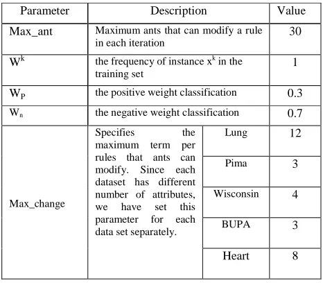
Table 2 shows parameters specification that we have used in our computer simulations for Fc-AntMiner.

Comparative performance of Fc-AntMiner is evaluated using ten-fold cross-validation test [1] which data set is divided into ten partitions, and Fc-AntMiner is run ten times, using a different partition as test set each time, with the other nine as training set. The classification rate is being calculated according to equation (17).

U}w~~Tw~{b Mw (17)

Where

TP: true positives, the number of cases in our training set covered by the rule that have the class predicted by the rule.

FP: false positives, the number of cases covered by the rule that have a class different from the class predicted by the rule FN: false negatives, the number of cases that are not covered by the rule but that have the class predicted by the rule.

[image:5.595.308.541.128.332.2]

TN: true negatives, the number of cases that are not covered by the rule and that do not have the class predicted by the rule.

Table 2. Parameter specification in computer simulation

Parameter Description Value

Max_ant Maximum ants that can modify a rule in each iteration

30

Wk _{the frequency of instance x}k_{in the}

training set

1

WP the positive weight classification 0.3

Wn the negative weight classification 0.7

Max_change

Specifies the maximum term per rules that ants can modify. Since each dataset has different number of attributes, we have set this parameter for each data set separately.

Lung 12

Pima 3

Wisconsin 4

BUPA 3

Heart 8

Also, precision measures of how many of the correctly classified samples are positive samples and Recall measures the of how many of positive sample are correctly classified. Precision and Recall are computed by following equations:

Precision 18

Recall 19

Precision and Recall stand in opposition to one another [22]. As precision goes up, recall usually goes down (and vice versa). F-Measure is a trade-off between Precision and Recall. It is the harmonic-mean of Precision and Recall and takes account of both measures. It is computed according to equation (20).

F X Measure 2 @ Precision @ Recall_{Precision 1 Recall 20}

[image:5.595.308.553.543.728.2]

Tables 2-6 show the mean classification rate, Precision, Recall and F-Measure for the generated rules by Fc-AntMiner and several well-known methods.

Table 3. Wisconsin Breast Cancer data set.

Method Classification

Rate Precision Recall F-Measure

SVM 0.967096 0.967 0.967 0.967

NaiveBayes 0.959943 0.962 0.96 0.96

C4.5 0.945637 0.946 0.946 0.946

NN 0.958512 0.959 0.959 0.959

KNN 0.951359 0.951 0.951 0.951

Decision

Table 0.95422 0.954 0.954 0.954 BayesNet 0.959943 0.962 0.96 0.96

(6)

Table 4. Pima Indian Diabetes data set.

SVM 0.77343 0.769 0.773 0.763

NaiveBayes 0.76302 0.759 0.763 0.76

C4.5 0.73828 0.735 0.738 0.736

NN 0.753906 0.75 0.754 0.751

KNN 0.70182 0.696 0.702 0.698

Decision

Table 0.71224 0.706 0.712 0.708 BayesNet 0.74349 0.741 0.743 0.742

Fc-AntMiner 0.83333 0.848 0.831 0.839

Table 4. Lung cancer data set.

SVM 0.481481 0.466 0.481 0.471

NaiveBayes 0.703704 0.704 0.704 0.704

C4.5 0.48148 0.342 0.481 0.400

NN 0.518519 0.528 0.519 0.522

KNN 0.481481 0.421 0.481 0.444

Decision

Table 0.518519 0.494 0.519 0.502 BayesNet 0.592593 0.575 0.593 0.58

Fc-AntMiner 0.62963 0.736 0.732 0.739

Table 5. BUPA Liver data set.

Table 6. Heart Disease data set.

It can be seen Fc-AntMiner has the considerable results and its performance is competitive with famous methods such as SVM, NN.

The following table shows the mean number of effective features in each data set. Fc-AntMiner detected these attributes by using the new heuristic information which we have proposed

(Section 3.1.1). The other features are recognized as don’t care features.

Table 7. Effective features.

Data set Number of attributes

Number of effective Attributes

Lung 56 18.354

Pima 8 3.240

Wisconsin 10 4.179

BUPA 7 3.196

Heart 13 7.2

Also, table 8 shows the computation time to build each classifier.

Table 8. time taken to build classifier

Data Set Non-Parallel Parallel

Wisconsin 6.72 3.74

Pima 10.78 6.64

Bupa 11.45 7.93

Heart 5.73 3.01

Lung 4.69 2.69

5. CONCLUSION

This paper presents a mixture of Ant Colony Optimization and Fuzzy Logic to medical classification, named Fc-AntMiner. In training stage, we have proposed a cooperative ACO algorithm for fuzzy rule learning. Then in testing stage, a fuzzy inference engine is used to classify test patterns. The main new features of the presented algorithm are as follows:

SVM 0.582609 0.757 0.583 0.432

Naïve

Bayes 0.565217 0.623 0.565 0.555

C4.5 0.686957 0.683 0.687 0.680

NN 0.715942 0.714 0.716 0.711

KNN 0.628986 0.63 0.629 0.629

Decision

Table 0.576812 0.561 0.577 0.558 BayesNet 0.562319 0.535 0.562 0.522

Fc-AntMine

r

0.678261 0.675 0.678 0.675

Method Classification Rate

Precision Recall F-Measure

SVM 0.84074 0.841 0.841 0.840

NaiveBayes 0.83333 0.833 0.833 0.833

C4.5 0.76666 0.766 0.767 0.767

NN 0.78148 0.784 0.781 0.782

KNN 0.75185 0.753 0.752 0.752

Decision Table

0.84814 0.848 0.848 0.848

BayesNet 0.81111 0.811 0.811 0.811

Fc-AntMiner

(7)