Distributed Modified Extremal Optimization for Reducing Crossovers in Reconciliation Graph

Distributed Modified Extremal Optimization for

Reducing Crossovers in Reconciliation Graph

Keiichi Tamura, Hajime Kitakami, and Akihiro Nakada

Abstract—To determine the mechanism of molecular evo-lution, a reconciliation graph is constructed from two het-erogeneous trees, which are referred to as ordered trees. In the reconciliation graph, the leaf nodes of the two ordered trees face each other. Furthermore, leaf nodes with the same label name are connected to each other by an edge. To carry out reconciliation work efficiently, it is necessary to find the state with the minimum number of crossovers of edges between leaf nodes. Reducing crossovers in a reconciliation graph is a combinatorial optimization problem. In this paper, we propose a novel bio-inspired algorithm called distributed modified extremal optimization (DMEO). This algorithm is a hybrid of population-based modified extremal optimization (PMEO) and the distributed genetic algorithm model that is used for reducing crossovers in a reconciliation graph. We have evaluated DMEO using actual data sets. DMEO shows better performance compared with PMEO.

Index Terms—extremal optimization, distributed genetic al-gorithm, evolutionary computation, reconciliation graph

I. INTRODUCTION

M

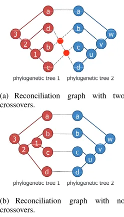
OLECULAR biologists need to carry out reconcilia-tion work [1], [2], [3], [4] in order to determine the mechanism of molecular evolution. In reconciliation work, the relation between two heterogeneous phylogenetic trees and the relation between a phylogenetic tree and a taxonomic tree are compared. To compare two trees, we construct a graph called a reconciliation graph that consists of two phy-logenetic trees or a phyphy-logenetic tree and a taxonomic tree. Phylogenetic trees and taxonomic trees in a reconciliation graph are referred to as ordered trees. The leaf nodes of these ordered trees face each other. Moreover, leaf nodes with the same label name are connected to each other by an edge. To carry out reconciliation work efficiently, it is necessary to find the state with the minimum number of crossovers of edges between leaf nodes in the reconciliation graph.

In Fig. 1, phylogenetic tree 1 and phylogenetic tree 2 are inferred from different molecular sequences with four identical species “a,” “b,” “c,” and “d.” The leaf nodes of phylogenetic tree 1 and those of phylogenetic tree 2 face each other. Leaf nodes representing the same species are connected to each other. The reconciliation graph shown in Fig. 1(a) has two crossovers. If we reduce crossovers in the reconciliation graph, we can obtain the reconciliation graph shown in Fig. 1(b), which has no crossovers.

Reducing crossovers in a reconciliation graph is a com-binatorial optimization problem. The number of combina-tions increases exponentially as the number of leaf nodes increases. There are some heuristics [5], [6] that can be used for reducing crossovers in a reconciliation graph, and

K.Tamura, H.Kitakami, and A.Nakada are with Graduate School of Information Sciences, Hiroshima City University, 3-4-1, Ozuka-Higashi, Asa-Minami-Ku, Hiroshima 731-3194 Japan, corresponding e-mail: ([email protected]).

a a

a a

d b

3 d b w

2 _{b c} v

1 b

u c

c d

c d

h l ti t 1 h l ti t 2 phylogenetic tree 1 phylogenetic tree 2

(a) Reconciliation graph with two crossovers.

a a

a a

b b

3 ₁ b b w

2 1 _{cc c} v

u c

d d

d d

h l ti t 1 h l ti t 2 phylogenetic tree 1 phylogenetic tree 2

(b) Reconciliation graph with no crossovers.

Fig. 1. Examples of reconciliation graphs ((a) shows a reconciliation graph that has two crossovers, and (b) shows a reconciliation graph that has no crossovers).

they use a genetic algorithm(GA)[7], extremal optimization (EO) [8], [9], [10], and modified EO (MEO)[11]. In our previous study[12], we proposed population-based modified extremal optimization (PMEO), which is a combination of a population-based approach and MEO.

PMEO shows better performance compared with MEO. However, it is difficult to maintain diversity at the end of alternation of generations. To overcome this difficulty, this paper proposes a novel extremal optimization model called distributed modified extremal optimization (DMEO) for reducing crossovers in a reconciliation graph. DMEO is a hybrid of PMEO and the distributed genetic algorithm (DGA) model [13], [14]. In the DGA model, we divide a population into two or more sub-populations and each sub-population evolves individually. Therefore, DMEO can maintain diversity at the end of alternation of generations.

The main contributions of this study are as follows:

• Distributed modified extremal optimization (DMEO) is proposed. DMEO is a hybrid bio-inspired algorithm that combine PMEO and DGA. Many studies [8], [9], [10], [15], [16], [17], [18] have applied EO to com-binatorial optimization problems such as the traveling salesman problem, graph partitioning problem, and im-age rasterization. Recently, some studies [19], [20] have focused on integrating a population-based approach in EO. To the best of our knowledge, there is no study on population-based EO involving the use of the distributed genetic algorithm model.

[image:1.595.364.488.160.376.2]

a a

a a

v₁₄ v₂₄

d b

v

11 v21

3 v₁₂ v w

15

v₂₂ v

25

2 v _{b c} v

13 v23

1 v₁₆ v₂₆ u

c d

c d

v₁₇ v₂₇

phylogenetic tree 1 phylogenetic tree 2

a b c d

1 0 0 0 0 0 0 1

a d 0 0 0 1

0 1 0 0

d b

CM = 0 1 0 0 0 0 1 0

b c 0 0 1 0

[image:2.595.68.213.53.122.2]

c

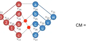
Fig. 2. Problem definition.

MDEO for reducing crossovers in a reconciliation graph. Moreover, we evaluated DMEO using two actual data sets for experiments. Experimental results shows that DMEO outperforms PMEO.

The rest of the paper is organized as follows. Section II presents the problem definition. Section III explains PMEO. Section IV proposes DMEO. Section V presents experimen-tal results, and Section VI concludes the paper.

II. PROBLEMDEFINITION

A reconciliation graph (RG) consists of two ordered trees,

OT1= (V1, E1)andOT2= (V2, E2), whereV1 andV2 are

finite sets of nodes and E1 and E2 are finite sets of edges.

A node that has no child nodes is a leaf node. The leaf node sets ofOT1andOT2 are denoted by L1∈V1 andL2∈V2,

respectively. If the number of species is n, the number of leaf nodes is n. A leaf node has a label name, which is a species’ name. The label name set is denoted byLleaf.

In the reconciliation graph,OT1andOT2are located face

to face. If a leaf node of OT1 has the same label name as

that of OT2, then the two leaf nodes are connected to each

other. In Fig.2, phylogenetic tree 1 isOT1and phylogenetic

tree 2 isOT2. The leaf node setL1has four nodes,v14,v15,

v16, andv17. Similarly,L2has four nodes,v24,v25,v26, and

v27. There are four label names inLleaf, “a,” “b,” “c,” and

“d.” Two leaf nodesv14 andv24 are connected because they

have the same label name “a.”

LetOL1 andOL2 be the order lists of leaf nodes:

OL1= [ol1,1, ol1,2,· · ·, ol1,n](ol1,i∈L1,L(ol1,i)∈Lleaf),

OL2= [ol2,1, ol2,2,· · ·, ol2,n](ol2,i∈L2,L(ol2,i)∈Lleaf),

where functionL returns the label name of an input node. The functionC(M)returns the number of crossovers:

C(M) =Xmj,βmk,α[1≤j < k≤n,1≤α < β≤n], (1)

where mi,j is (i, j)th-element of the connection matrix M

that is defined as

mi,j=

1 if L(ol1,i) = L(ol2,j),

0 otherwise. (2)

In Fig. 2, OL1 is given by OL1 = [v14, v15, v16, v17].

Similarly, there are four leaf nodes in phylogenetic tree 2,

ol2,1 = v24, ol2,2 = v25, ol2,3 = v26, and ol2,4 = v27.

ThereforeOL2is given byOL2= [v24, v25, v26, v27]. Fig. 2

also showsM. For example, the(0,0)th-elementm0,0 is 1

becauseL(v14)equalsL(v24). Similarly, the(1,1)th-element

m1,1 is 0 becauseL(v15)does not equalL(v25).

The task of reducing crossovers in the reconciliation graph is defined as follows:

min: C(M),

subject to: (1)M is the connection matrix of theRG,

(2) There are no crossovers on edges between non-leaf nodes in the RG.

There should be no crossovers on edges between non-leaf nodes in the reconciliation graph. For this constraint, we need to change order of leaf nodes by changing the order of child nodes in intermediate nodes. We cannot change the order between v15 andv17 (Fig. 2) because it will lead to

the presence of crossovers on edges between non-leaf nodes. If we want to change the order between v15 and v17, it is

necessary to replacev15 andv13, which are child nodes of

v12. If we replacev15 andv13, the number of crossovers in

the reconciliation graph becomes zero, andOL1 is changed

toOL1= [v14, v16, v17, v15].

III. POPULATION-BASEDMODIFIEDEXTREMAL

OPTIMIZATION

EO[8], [9], [10] follows the spirit of the Bak-Sneppen model, updating variables that have one of the worst values in a solution and replacing them by random values without ever explicitly improving them. EO divides an individualIinton

componentsOi(1≤i≤n). Letλibe the fitness value ofOi.

First, EO selectsOworst, which has the worst fitness value.

Second, the state of componentOworstis changed at random.

Henceforth, selection and change state of a component are repeated. The component with the worst fitness value has a high possibility that the fitness value of it will become better by changing state. Consequently, the fitness value of the individual also gets better because the fitness value of the component with worst fitness value gets better.

Modified EO (MEO) [11] generates two or more neighbor individuals as candidates for the next generation individual. The best neighbor individual among the candidates is se-lected as the next generation individual. Moreover, MEO uses roulette selection to select a component. First, MEO selectsOselected with roulette selection. The selection rates

of roulette selection are reciprocals of fitness values with components. Second, MEO generates new individualI′_from

Iby changing the state ofOselected. Third, the generatedI′

is stored into Candidates. Finally, MEO selects the best individual fromCandidates.

Population-based MEO (PMEO) [12] involves a population-based approach. There are two or more individuals in a population. Alternation of generation is repeatedly performed for every individual by using MEO. To improve the search efficiency, individuals copy a sub-structure of an individual that has good sub-sub-structures at each alternation of generations. This operation resembles the crossover operation in genetic programing (GP). However, one side only copies a sub-structure of another side. Copying of good sub-structures leads to a high probability of generation of a good individual. As a result, efficient search can be performed by maintaining diversity.

IV. DISTRIBUTEDMODIFIEDEXTREMALOPTIMIZATION

A. Main Concept

DMEO is a hybrid of PMEO and DGA model. DMEO di-vides the entire population into two or more sub-populations. A sub-population evolves individually by PMEO. Moreover, from each sub-population, some individuals are selected and transferred to another sub-population. In return, the same number of migrants are received from another sub-population. DMEO repeats the following two steps:

(1) Sub-populations should be made to evolve through one or more generations by using PMEO.

(2) Some individuals of a sub-population are migrated to another sub-population.

Each population evolves individually. Each sub-population converges to the separate best solution. Therefore, DMEO can maintain diversity at the end of alternation of generations.

B. Definition of Individual and Component

A reconciliation graph is defined as an individual. A component of an individual is defined as a pair of leaf nodes with the same label name:

Oi ={ol1,i, ol2,δ(i)} (L(ol1,i) =L(ol2,δ(i))). (3)

Letol1,ibe a leaf node ofOL1andol2,δ(i)be a leaf node of

OL2. The functionδ(i) returns the subscript number of an

element of OL2 whose label name is the same as the label

name of ol1,i. To change the state of Oi, it is necessary to

change the order of child nodes of ancestor nodes ofol1,ior

ol2,δ(i). Here,AS(T, lname)is a set of ancestor nodes of a

leaf node inT that has the label namelname.

The number of crossovers between ol1,i and ol2,δ(i) is

denoted by C(M, i). The following are the definitions of

C(M, i)and the fitness valueλi ofOi:

λi =

C(M)− C(M, i)

C(M) , (4)

C(M, i) =

n X

l=i+1 δ(i)−1

X

m=1

ml,m

2 +

i−1 X

l=1 n X

m=δ(i)+1

ml,m

2 .(5) In Fig. 2, there are four components,O1={ol1,1, ol2,1}(= {v14, v24}), O2 = {ol1,2, ol2,4}(= {v15, v27}), O3 = {ol1,3, ol2,2}(= {v16, v25}), and O4 = {ol1,4, ol2,3}(= {v17, v26}), with δ(1) = 1, δ(2) = 4, δ(3) = 2, and

δ(4) = 3. The fitness values of the components are λ1= 1,

λ2= 1/2,λ3= 3/4, andλ4= 3/4.

C. Algorithm

The algorithm of DMEO for reducing crossovers in a reconciliation graph consists of two steps: (1) Evolution Step and (2) Migration Step (Algorithm 1). First, an initial population divided to p sub-populations (p is the number of sub-populations). In the Evolution Step (step 5), all sub-populations are made to evolve through m generations by using the function PMEO(SubPi, m) (m is migration

interval). In Migration Step (step 6), some individuals of a sub-population are migrated to another sub-population. Finally, the best individual from all sub-populations (step 7 and step 8).

Algorithm 1 DMEO

1: Generate initial populationPinit at random. 2: Ibest←BEST(Pinit)

3: Divide Pinit intopsub-populationsSubPi. 4: fori= 1 tomax generations/mdo

5: (Evolution Step) For all populations, sub-population SubPi should be made to evolve

through m generations by using the function PMEO(SubPi, m).

6: (Migration Step) For all sub-populations, migrate some individuals of a population to another sub-population.

7: ifF(BEST(SubP1∩ · · · ∩SubPp))>F(Ibest)then 8: Ibest←BEST(SubP1∩ · · · ∩SubPp)

9: end if 10: end for

Algorithm 2 PMEO(P,m)

1: fori= 1 tomdo 2: for allI∈P do

3: Evaluate fitness valueλi of each componentOi of

I.

4: C←φ

5: n←0

6: while n < num of candidates do

7: Select Oselected by roulette selection (selection

rates are the reciprocal of fitness values with components).

8: C←C∪GNI(I, Oselected)

9: n←n+ 1

10: end while

11: I←BEST(C)

12: end for 13: CSS(P)

14: end for

D. Evolution Step

In the Evolution Step, all sub-populations are made to evolve throughmgenerations by using the functionPMEO (Algorithm 2). First, for each individual, the state of the individuals in P is changed by using MEO. Second, the functionCSS copies a good sub-structure of an individual to another individual.

In the MEO steps, for each individual, the following steps are executed. Initially, the function evaluates the fitness value

λi (step 3). Next, the following three steps are repeated

whilenis less thannum of candidates. First, component

Oselected inI is selected by using the roulette selection (step

7). Second, the function generates an neighbor individual fromIwith the functionGNI. The functionGNIgenerates a neighbor individual by changing the state of component

Oselected. Third, the neighbor individual is stored inC(step

8). Finally, the best individual in C is selected and I is replaced by it (step 11).

The state ofOselected is changed by changing the order

of child nodes in an intermediate node that is an ances-tor node of Oselected. The processing steps of GNI are

TABLE I DATA SETS

Taxonomic tree Phylogenetic tree

Number of nodes Number of leaf nodes Number of nodes Number of leaf nodes

Housekeeping 241 40 79 40

M oss 290 207 394 207

Algorithm 3 CSS(P)

1: Select individualSI∈P by roulette selection (selection rates are the fitness values of components).

2: for allI∈P, I6=SI do 3: fori= 1tondo

4: Calculate the difference diffi between the fitness

value of Oi inSIand the fitness value ofOj inI,

whereOi andOj have the same label name. 5: end for

6: SelectOselected by roulette selection (selection rates

arediffi).

7: A← AS(T1,L(Oselected))orAS(T2,L(Oselected))

8: C←φ

9: for alla∈A do

10: Generate a new individual I′ _{from I by changing} the order of child nodes in a.

11: C←C∪I′ 12: end for

13: I←BEST(C) 14: end for

node a is selected at random from A. Finally, the order of the child nodes in a is changed. Suppose that the selected component is O2 in Fig. 2. The function AS(T1,L(O2))

returns{v12, v11} andAS(T2,L(L2))returns{v22, v21}. If

Ancestors={v12, v11} andv12 is selected asa, the order

of child nodes inv12is changed. In this case, order of node

v15 andv13 are changed. As a result, a new individualI′ is

obtained by the change of state.

Algorithm 3 shows the function CSS. At the beginning, an individualSI inP is selected by roulette selection (step 1). Each individual ofP copies a sub-structure ofSIby the following steps. First, the function calculates the difference

dif fi between the fitness value ofOi ofSI and the fitness

value of Oj of I, where Oi and Oj have the same label

name (steps 3, 4, and 5). Second, Oselected is selected by

roulette selection (step 6). Next, AS(T1,L(Oselected)) or AS(T2,L(Oselected)) is stored in A (step 7). Then, for all

a∈A, a new individualI′ _{is generated fromIby changing} the order of child nodes in a, and I′ _{is stored in C (steps} 9, 10, 11, and 12). Finally, the function selects the best individual fromC (step 13).

E. Migration Step

In the Migration Step, some individuals of a sub-population are migrated to another sub-sub-population. The dis-tributed genetic algorithm model requiresnumber of sub−

populations, migration rate, migration interval, and

migration model. The first three items are user-given parameters. The last item consists of two things:

selection method and topology. The method used for the selection of individuals for migration is referred as

selection method. The structure of the migration of in-dividuals between sub-populations is referred as topology. In this study, we use uniform random selection as the

selection method. Moreover, the proposed algorithm uses the random ring migration topology. The most basic migra-tion topology is the ring migramigra-tion topology. In this topology, individuals are transferred between directionally adjacent sub-populations. In the random ring migration topology, an arrival sub-population to which individuals are to be migrated is decided at random.

V. PERFORMANCEEVALUATION

We performed four experiments for evaluating the perfor-mance of DMEO. In the experiments, the two data sets listed in Table I are used. TheHousekeepingdata set consists of a phylogenetic tree of the housekeeping gene and its taxonomic tree. TheM oss data set consists of a phylogenetic tree of the rps4 gene and its taxonomic tree. The number of species in the Housekeepingdata set is 40 and that in the M oss

data set is 207.

Experiment 1 measured the number of crossovers of the best individual at each generation to compare DMEO and PMEO. Experiment 2 also measured the number of crossovers of the best individual at each elapsed time to compare DMEO and PMEO. Experiment 3 measured fre-quency of the number of crossovers of best individuals in fixed generations. Experiment 4 measured the number of crossovers of the best individual at each generation by changing the number of sub-populations.

In PMEO and DMEO, the number of individu-als in the population was set to 100. The user pa-rameter num of candidates was set to 100 and m

was set to 10000 in PMEO. In DMEO, the user parameter num of candidates, migration interval(m),

number of sub−populations(p), andmigration ratewere set to be 100, 10, 5 and 0.05, respectively. The number of individuals in a sub-population is 20. The number of crossovers was the average of three trials.

Experiment 1

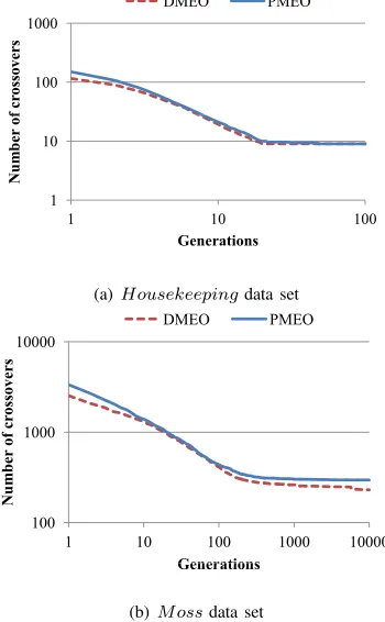
In Experiment 1, we measured the number of crossovers of the best individual in each generation. Figure3(a) and Figure3(b) show the number of crossovers (vertical axis: the number of crossovers, horizontal axis: generations). Fig. 3(a) and Fig. 3(b) show that the number of crossovers of DMEO in each generation was smaller than that in the case of PMEO. DMEO showed better performance compared with PMEO.

100 1000

f

cr

o

ss

o

v

er

s

DMEO PMEO

1 10

1 10 100

N

u

m

b

er

o

f

Generations Generations

(a)Housekeepingdata set

1000 10000

f

cr

o

ss

o

v

er

s

DMEO PMEO

100 1000

1 10 100 1000 10000

N

u

m

b

er

o

f

Generations Generations

[image:5.595.338.506.53.339.2]

(b)M ossdata set

Fig. 3. Experiment 1 ((a) and (b) shows the number of crossovers of the best individual) .

value of a individual will not be improved in the end of alternation of generations.

Experiment 2

In Experiment 2, we measured the number of crossovers of the best individual at different time instants. The computation time of DMEO was longer than that in the case of PMEO because the former included the Migration Step. Therefore, it was necessary to compare the number of crossovers for the same computation time.

Fig. 4(a) and Fig. 4(b) show the number of crossovers at different time instants (vertical axis: the number of crossovers, horizontal axis: processing time). The number of crossovers of DMEO becomes smaller than that of PMEO at the end of alternation of generations.

Experiment 3

The number of crossovers of the best individual was measured 100 times for the 10,000th alternation generation. Figure5(a) and Figure5(b) show frequency of the number of crossovers whenHousekeepingdata set is used. The num-ber of crossovers of the optimal solution ofHousekeeping

data set is 9. Both of them can obtain the best solution by 100%. Fig. 6(a) and Fig. 6(b) show the frequency of the number of crossovers for theM oss data set. In DMEO, all the numbers of crossovers of optimal solutions were between 200 and 299. On the other hand, they were distributed between 200 and 400 for PMEO. Above all, although 90% of optimal solutions were between 200 and 249 in the case of DMEO, only a few optimal solutions were obtained between 200 and 249 in the case of MEO.

100 1000

f

cr

o

ss

o

v

er

s

DMEO PMEO

1 10

0.1 1 10 100

N

u

m

b

er

o

f

Processing time(sec) Processing time(sec)

(a)Housekeepingdata set

1000 10000

f

cr

o

ss

o

v

er

s

DMEO PMEO

100 1000

1 10 100 1000 10000 100000

Num

b

er

o

f

Processing time(sec) Processing time(sec)

(b)M ossdata set

Fig. 4. Experiment 2 ((a) and (b) shows the number of crossovers of the best individual).

Experiment 4

In Experiment 4, we changed the number of sub-populations in DMEO. Fig. 7 shows the results of Experiment 4 usingM ossdata set. When the number of sub-populatins is four, it has fallen into the local optimal solutions. On the other hand, when the number of sub-pouplations is five or ten, convergence is not early. Therefore, they can obtain better solutions.

VI. CONCLUSION

This paper proposes distributed modified extremal opti-mization (DMEO) for reducing crossovers in a reconciliation graph. The proposed algorithm is a bio-inspired algorithm of population-based modified extremal optimization (PMEO) and the distributed genetic algorithm model. We have evalu-ated DMEO by using actual data sets. Experimental results show that DMEO is better performance compared with PMEO. In the future work, we will develop extended DMEO for making it applicable to other combination optimization problems.

ACKNOWLEDGMENT

This work was supported in part by a Grant-in-Aid for Young Research (B) (No.23700124) from the Ministry of Education, Culture, Sports, Science and Technology in Japan and a Grant-in-Aid for Scientific Research (C) (2) (No.20500137) from the Japanese Society for the Promotion of Science, Japan.

REFERENCES

[image:5.595.80.255.60.343.2]

40 00% 60.00% 80.00% 100.00% 40 50 60 70 80 90 100 iv e fr e qu e nc y e q u e n cy 0.00% 20.00% 40.00% 60.00% 80.00% 100.00% 0 10 20 30 40 50 60 70 80 90 100

9 10 11 12 13 14 15

C u m u la ti v e fr e qu e nc y F req u en cy

Number of crossovers

0.00% 20.00% 40.00% 60.00% 80.00% 100.00% 0 10 20 30 40 50 60 70 80 90 100

9 10 11 12 13 14 15

C u m u la ti v e fr e qu e nc y F req u en cy

Numberofcrossovers

(a) PMEO 40 00% 60.00% 80.00% 100.00% 40 50 60 70 80 90 100 iv e fr e qu e nc y e q u e n cy 0.00% 20.00% 40.00% 60.00% 80.00% 100.00% 0 10 20 30 40 50 60 70 80 90 100

9 10 11 12 13 14 15

C u m u la ti v e fr e qu e nc y F req u en cy

Number of crossovers

0.00% 20.00% 40.00% 60.00% 80.00% 100.00% 0 10 20 30 40 50 60 70 80 90 100

9 10 11 12 13 14 15

C u m u la ti v e fr e qu e nc y F req u en cy

Numberofcrossovers

[image:6.595.340.514.55.184.2]

(b) DMEO

Fig. 5. Experiment 3 (Housekeepingdata set).

60.00% 80.00% 100.00% 50 60 70 80 90 100 v e F re q u e n cy q u e n cy 0.00% 20.00% 40.00% 0 10 20 30 40

200249 250299 300349 350400

C u m u la ti v F re q

Numberofcrossovers

(a) PMEO 60.00% 80.00% 100.00% 50 60 70 80 90 100 v e F re q u e n cy q u e n cy 0.00% 20.00% 40.00% 0 10 20 30 40

200249 250299 300349 350400

C u m u la ti v F re q

Numberofcrossovers

(b) DMEO

Fig. 6. Experiment 3 (M ossdata set).

[2] R. Page, “Maps between trees and cladistic analysis of historical associations among genes, organisms, and areas,”Systematic Biology, vol. 43, pp. 58–77, 1994.

[3] R. D. M. Page and M. A. Charleston, “Reconciled trees and incon-gruent gene and species trees,”Discrete Mathametics and Theoretical

Computer Science, vol. 37, pp. 57–70, 1997.

[4] R. D. M. Page, “Genetree: comparing gene and species phylogenies using reconciled trees,”Bioinformatics, vol. 14, no. 9, pp. 819–820, 1998.

[5] H. Kitakami and M. Nishimoto, “Constraint satisfaction for reconciling heterogeneous tree databases,” inProceedings of DEXA 2000, 2000, pp. 624–633. 260 280 300 cr os so v e rs

p=4 p=5 p=10

200 220 240

0 5000 10000

N u m b e r o f c

0 5000 10000

[image:6.595.86.263.61.339.2]

Generations

Fig. 7. Experiment 4 (M ossdata set).

[6] H. Kitakami and Y. Mori, “Reducing crossovers in reconciliation graphs using the coupling cluster exchange method with a genetic algorithm,”Active Mining, IOS press, vol. 79, pp. 163–174, 2002. [7] D. E. Goldberg, Genetic Algorithms in Search, Optimization, and

Machine Learning. Addison-Wesley Professional, January 1989.

[8] S. Boettcher and A. G. Percus, “Extremal optimization: Methods derived from co-evolution,” in Proceedings of GECCO 1999, 1999, pp. 825–832.

[9] S. Boettcher and A. Percus, “Nature’s way of optimizing,”Artificial

Intelligence, vol. 119, no. 1-2, pp. 275–286, 2000.

[10] S. Boettcher, “Extremal optimization: heuristics via coevolutionary avalanches,” Computing in Science and Engineering, vol. 2, no. 6, pp. 75–82, 2000.

[11] K. Tamura, Y. Mori, and H. Kitakami, “Reducing crossovers in reconciliation graphs with extremal optimization (in japanese),”

Trans-actions of Information Processing Society of Japan, vol. 49, no.

4(TOM 20), pp. 105–116, 2008.

[12] N. Hara, K. Tamura, and H. Kitakami, “Modified eo-based evolu-tionary algorithm for reducing crossovers of reconciliation graph,” in

Proceedings of NaBIC 2010, 2010, pp. 169–176.

[13] R. Tanese, “Distributed genetic algorithms,” inProceedings of the 3rd

International Conference on Genetic Algorithms, 1989, pp. 434–439.

[14] T. C. Belding, “The distributed genetic algorithm revisited,” in

Pro-ceedings of the 6th International Conference on Genetic Algorithms,

1995, pp. 114–121.

[15] S. Meshoul and M. Batouche, “Robust point correspondence for image registration using optimization with extremal dynamics,” in

Proceedings of DAGM-Symposium 2002, 2002, pp. 330–337.

[16] S. Boettcher and A. G. Percus, “Extremal optimization at the phase transition of the 3-coloring problem,” Physical Review E, vol. 69, 066703, 2004.

[17] T. Zhou, W.-J. Bai, L.-J. Cheng, and B.-H. Wang, “Continuous extremal optimization for lennard-jones clusters,”Physical Review E, vol. 72, 016702, 2005.

[18] J. Duch and A. Arenas, “Community detection in complex networks using extremal optimization,” Physical Review E, vol. 72, 027104, 2005.

[19] Y. Chen, K. Zhang, and X. Zou, “A population-based hybrid ex-tremal optimization algorithm,” inProceedings of the 7th international conference on Intelligent Computing: bio-inspired computing and

applications, 2011, pp. 410–417.

[image:6.595.81.265.377.620.2]