Word Translation Disambiguation Using Bilingual Bootstrapping

Bilingual Bootstrapping

Hang Li

_{Cong Li}

Microsoft Research Asia Microsoft Research Asia

This article proposes a new method for word translation disambiguation, one that uses a machine-learning technique called bilingual bootstrapping. In machine-learning to disambiguate words to be trans-lated, bilingual bootstrapping makes use of a small amount of classified data and a large amount of unclassified data in both the source and the target languages. It repeatedly constructs classi-fiers in the two languages in parallel and boosts the performance of the classiclassi-fiers by classifying unclassified data in the two languages and by exchanging information regarding classified data between the two languages. Experimental results indicate that word translation disambiguation based on bilingual bootstrapping consistently and significantly outperforms existing methods that are based on monolingual bootstrapping.

1. Introduction

We address here the problem of word translation disambiguation. If, for example, we were to attempt to translate the English nounplant, which could refer either to a type of factory or to a form of flora (i.e., in Chinese, either to [gongchang] or to [zhiwu]), our goal would be to determine the correct Chinese translation. That is, word translation disambiguation is essentially a special case of word sense disambiguation (in the above example,gongchangwould correspond to the sense offactoryand zhiwu to the sense offlora).1

We could view word translation disambiguation as a problem of classification. To perform the task, we could employ a supervised learning method, but since to do so would require human labeling of data, which would be expensive, bootstrapping would be a better choice.

Yarowsky (1995) has proposed a bootstrapping method for word sense disam-biguation. When applied to translation from English to Chinese, his method starts learning with a small number of English sentences that contain ambiguous English words and that are labeled with correct Chinese translations of those words. It then uses these classified sentences as training data to create a classifier (e.g., a decision list), which it uses to classify unclassified sentences containing the same ambiguous words. The output of this process is then used as additional training data. It also adopts the one-sense-per-discourse heuristic (Gale, Church, and Yarowsky 1992b) in classifying unclassified sentences. By repeating the above process, an accurate classifier for word translation disambiguation can be created. Because this method uses data in a single language (i.e., the source language in translation), we refer to it here as monolingual bootstrapping (MB).

∗5F Sigma Center, No. 49 Zhichun Road, Haidian, Beijing, China, 100080. E-mail:{hangli,i-congl}@ microsoft.com.

In this paper, we propose a new method of bootstrapping, one that we refer to as bilingual bootstrapping (BB). Instead of using data in one language, BB uses data in two languages. In translation from English to Chinese, for example, BB makes use of unclassified data from both languages. It also uses a small number of classified data in English and, optionally, a small number of classified data in Chinese. The data in the two languages should be from the same domain but are not required to be exactly in parallel.

BB constructs classifiers for English-to-Chinese translation disambiguation by re-peating the following two steps: (1) Construct a classifier for each of the languages on the basis of classified datain both languages, and (2) use the constructed classifier for each language to classify unclassified data, which are then added to the classified data of the language. We can use classified data in both languages in step (1), because words in one language have translations in the other, and we can transform data from one language into the other.

We have experimentally evaluated the performance of BB in word translation disambiguation, and all of our results indicate that BB consistently and significantly outperforms MB. The higher performance of BB can be attributed to its effective use of the asymmetric relationship between the ambiguous words in the two languages.

Our study is organized as follows. In Section 2, we describe related work. Specifi-cally, we formalize the problem of word translation disambiguation as that of classifi-cation based on statistical learning. As examples, we describe two such methods: one using decision lists and the other using naive Bayes. We also explain the Yarowsky disambiguation method, which is based on Monolingual Bootstrapping. In Section 3, we describe bilingual bootstrapping, comparing BB with MB, and discussing the re-lationship between BB and co-training. In Section 4, we describe our experimental results, and finally, in Section 5, we give some concluding remarks.

2. Related Work

2.1 Word Translation Disambiguation

Word translation disambiguation (in general, word sense disambiguation) can be viewed as a problem of classification and can be addressed by employing various supervised learning methods. For example, with such a learning method, an English sentence containing an ambiguous English word corresponds to an instance, and the Chinese translation of the word in the context (i.e., the word sense) corresponds to a classification decision (a label).

Many methods for word sense disambiguation based on supervised learning tech-nique have been proposed. They include those using naive Bayes (Gale, Church, and Yarowsky 1992a), decision lists (Yarowsky 1994), nearest neighbor (Ng and Lee 1996), transformation-based learning (Mangu and Brill 1997), neural networks (Towell and Voorhees 1998), Winnow (Golding and Roth 1999), boosting (Escudero, Marquez, and Rigau 2000), and naive Bayesian ensemble (Pedersen 2000). The assumption behind these methods is that it is nearly always possible to determine the sense of an ambigu-ous word by referring to its context, and thus all of the methods build a classifier (i.e., a classification program) using features representing context information (e.g., sur-rounding context words). For other related work on translation disambiguation, see Brown et al. (1991), Bruce and Weibe (1994), Dagan and Itai (1994), Lin (1997), Ped-ersen and Bruce (1997), Schutze (1998), Kikui (1999), Mihalcea and Moldovan (1999), Koehn and Knight (2000), and Zhou, Ding, and Huang (2001).

denote acontextword inE. (Throughout this article, we use Greek letters to represent ambiguous words and italic letters to represent context words.) LetTε denote the set of senses ofε, and lettεdenote a sense inTε. Leteεstand for an instance representing a context ofε, that is, a sequence of context words surroundingε:

eε= (eε,1,eε,2,. . .,(ε),. . .,eε,m),eε,i∈E, (i=1,. . .,m)

For the example presented earlier, we haveε=plant,Tε={1, 2}, where 1 represents the sensefactory and 2 the sense flora. From the phrase “. . .computer manufacturing plant and adjacent. . .” we obtain eε = (. . .computer, manufacturing, (plant), and, adjacent,. . .).

For a specificε, we define a binaryclassifier for resolving each of its ambiguities inTε in a general form as2

P(tε|eε), tε∈Tεand P(¯tε|eε), ¯_{tε=Tε− {tε}}

whereeεdenotes an instance representing a context ofε. All of the supervised learning methods mentioned previously can automatically create such a classifier. To construct classifiers using supervised methods, we need classified data such as those in Figure 1.

2.2 Decision Lists

Let us first consider the use of decision lists, as proposed in Yarowsky (1994). Let fε denote a feature of the context ofε. A feature can be, for example, a word’s occurrence immediately to the left of ε. We define many such features. For each feature fε, we use the classified data to calculate the posterior probability ratio of each sensetεwith respect to the feature as

λ(tε|fε) = P(tε|fε) P(¯tε|fε)

For each featurefε, we create a rule consisting of the feature, the sense

arg max

tε∈Tε

λ(tε|fε)

and the score

max

tε∈Tε

λ(tε|fε)

We sort the rules in descending order with respect to their scores, provided that the scores of the rules are larger than the default

max

tε∈Tε

P(tε) P(¯tε)

The sorted rules form an if-then-else type of rule sequence, that is, a decision list.3 _For

a new instance eε, we use the decision list to determine its sense. The rule in the list whose feature isfirstsatisfied in the context ofeεis applied in sense disambiguation.

2 In this article we always employ binary classifiers even there are multiple classes.

P1 . . .Nissan car and truckplant. . .(1)

P2 . . .computer manufacturingplantand adjacent. . .(1) P3 . . .automated manufacturingplantin Fremont. . .(1) P4 . . .divide life intoplantand animal kingdom. . .(2) P5 . . .thousands ofplantand animal species. . .(2) P6 . . .zonal distribution ofplantlife. . .(2)

. . . . . .

Figure 1

Examples of classified data (ε=plant).

2.3 Naive Bayesian Ensemble

Let us next consider the use of naive Bayesian classifiers. Given an instanceeε, we can calculate

λ∗(eε) =max

tε∈Tε

P(tε|eε) P(¯tε|eε) =maxtε∈Tε

P(tε)P(eε|tε) P(¯tε)P(eε|¯tε)

(1)

according to Bayes’ rule and select the sense

t∗(eε) =arg max

tε∈Tε

P(tε)P(eε|tε) P(¯tε)P(eε|¯tε)

(2)

In a naive Bayesian classifier, we assume that the words in eε with a fixed tε are independently generated from P(eε|tε)and calculate

P(eε|tε) =

m

i=1

P(eε,i|tε)

Here P(eε|tε)represents the conditional probability ofein the context ofε giventε. We calculate P(eε|¯tε) similarly. We can then calculate (1) and (2) with the obtained P(eε|tε)andP(eε|¯tε).

The naive Bayesian ensemble method for word sense disambiguation, as proposed in Pedersen (2000), employs a linear combination of several naive Bayesian classifiers constructed on the basis of a number of nested surrounding contexts4

P(tε|eε) = 1 h

h

i=1

P(tε|eε,i)

eε,1⊂ · · · ⊂eε,i· · · ⊂eε,h=eε(i=1,. . .,h)

The naive Bayesian ensemble is reported to perform the best for word sense disam-biguation with respect to a benchmark data set (Pedersen 2000).

2.4 Monolingual Bootstrapping

Since data preparation for supervised learning is expensive, it is desirable to develop bootstrapping methods. Yarowsky (1995) proposed such a method for word sense disambiguation, which we refer to as monolingual bootstrapping.

LetLεdenote a set of classified instances (labeled data) in English, each represent-ing one context ofε:

Lε={(eε,1,tε,1),(eε,2,tε,2),. . .,(eε,k,tε,k)}

tε,i∈Tε(i=1, 2,. . .,k)

and Uε a set of unclassified instances (unlabeled data) in English, each representing one context ofε:

Uε={eε,1,eε,2,. . .,eε,l}

The instances in Figure 1 can be considered examples ofLε. Furthermore, we have

LE=

ε∈E

Lε,UE=

ε∈E

Uε,T= ε∈E

Tε,

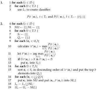
An algorithm for monolingual bootstrapping is presented in Figure 2. For a better comparison with bilingual bootstrapping, we have extended the method so that it

Input: E,T,LE,UE, Parameter:b,θ

Repeat the following processes until unable to continue

1. 1for each(ε∈E){ 2 for each(t∈Tε){

3 useLε to create classifier:

P(t|eε), t∈Tεand P(¯t|eε), ¯_{t∈Tε− {t};}}} 2. 4for each(ε∈E){

5 NU← {};NL← {}; 6 for each(t∈Tε){ 7 St← {};

8 Qt← {};}

9 for each(eε∈Uε){ 10 calculateλ∗(eε) =max

t∈Tε

P(t|eε) P(¯t|eε); 11 lett∗(eε) =arg max

t∈Tε

P(t|eε) P(¯t|eε); 12 if(λ∗(eε)> θ&t∗(eε) =t) 13 puteεinto St;}

14 for each(t∈Tε){

15 sorteε∈St in descending order ofλ∗(eε)and put the topb elements intoQt;}

16 for each(eε∈

tQt){

17 puteε intoNUand put(eε,t∗(eε))intoNL;} 18 Lε←LεNL;

19 Uε←Uε−NU;}

Figure 2

performs disambiguation for all the words in E. Note that we can employ any kind of classifier here.

At step 1, for each ambiguous wordεwe create binary classifiers for resolving its ambiguities (cf. lines 1–3 of Figure 2). At step 2, we use the classifiers for each word εto select some unclassified instances fromUε, classify them, and add them toLε(cf. lines 4–19). We repeat the process until all the data are classified.

Lines 9–13 show that for each unclassified instance eε, we classify it as having senset if t’s posterior odds are the largest among the possible senses and are larger than a thresholdθ. For each classt, we store the classified instances inSt. Lines 14–15

show that for each classt, we only choose the topbclassified instances in terms of the posterior odds. For each class t, we store the selected topbclassified instances inQt.

Lines 16–17 show that we create the classified instances by combining the instances with their classification labels.

After line 17, we can employ the one-sense-per-discourse heuristic to further clas-sify unclassified data, as proposed in Yarowsky (1995). This heuristic is based on the observation that when an ambiguous word appears in the same text several times, its tokens usually refer to the same sense. In the bootstrapping process, for each newly classified instance, we automatically assign its class label to those unclassified instances that also contain the same ambiguous word and co-occur with it in the same text.

Hereafter, we will refer to this method as monolingual bootstrapping with one sense per discourse. This method can be viewed as a special case of co-training (Blum and Mitchell 1998).

2.5 Co-training

Monolingual bootstrapping augmented with the one-sense-per-discourse heuristic can be viewed as a special case of co-training, as proposed by Blum and Mitchell (1998) (see also Collins and Singer 1999; Nigam et al. 2000; and Nigam and Ghani 2000). Co-training conducts two bootstrapping processes in parallel and makes them collaborate with each other. More specifically, co-training begins with a small number of classified data and a large number of unclassified data. It trains two classifiers from the classified data, uses each of the two classifiers to classify some unclassified data, makes the two classifiers exchange their classified data, and repeats the process.

3. Bilingual Bootstrapping

3.1 Basic Algorithm

Bilingual bootstrapping makes use of a small amount of classified data and a large amount of unclassified data in both the source and the target languages in translation. It repeatedly constructs classifiers in the two languages in parallel and boosts the performance of the classifiers by classifying data in each of the languages and by exchanging information regarding the classified data between the two languages.

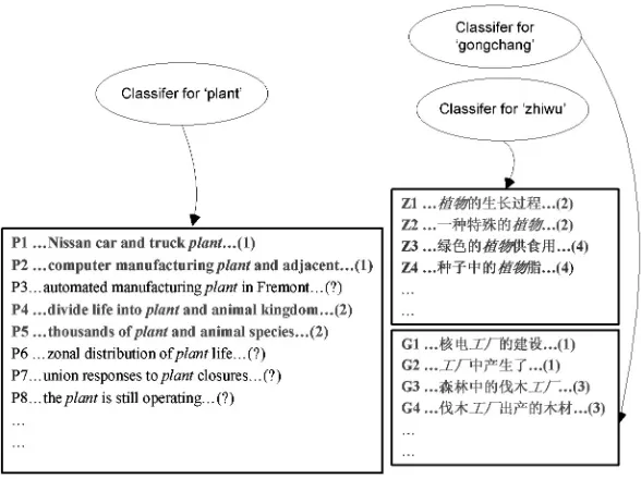
Figures 3 and 4 illustrate the process of bilingual bootstrapping. Figure 5 shows the translation relationship among the ambiguous wordsplant, zhiwu, andgongchang. There is a classifier for plantin English. There are also two classifiers, one each for zhiwu and gongchang, respectively, in Chinese. Sentences containing plant in English and sentences containingzhiwuandgongchangin Chinese are used.

Figure 3

Bilingual bootstrapping (1).

Figure 4

~

 

€



~

Figure 5

Example of translation dictionary.

not labeled. Bilingual bootstrapping uses labeled sentences P1, P4, G1, and Z1 to create a classifier forplantdisambiguation (between label 1 and label 2). It also uses labeled sentences Z1, Z3, and P4 to create a classifier forzhiwuand uses labeled sentences G1, G3, and P1 to create a classifier for gongzhang. Bilingual bootstrapping next uses the classifier forplantto label sentences P2 and P5 (Figure 4). It uses the classifier forzhiwu to label sentences Z2 and Z4, and uses the classifier for gongchangto label sentences G2 and G4. The process is repeated until we cannot continue.

To describe this process formally, letEdenote a set of words in English,Ca set of words in Chinese, andT a set of senses (links) in a translation dictionary as shown in Figure 5. (Any two linked words can be translations of each other.) Mathematically, T is defined as a relation between E and C, that is, T ⊆ E×C. Let ε stand for an ambiguous word inE, and γ an ambiguous word inC. Also letestand for a context word in E,c a context word inC, andta sense in T.

For an English wordε,Tε={t|t= (ε,γ), t∈T}represents the set ofε’s possible senses (i.e., its links), andCε={γ|(ε,γ)∈T}represents the Chinese words that can be translations ofε(i.e., Chinese words to whichεis linked). Similarly, for a Chinese word γ, letTγ ={t|t= (ε,γ),t∈T} andEγ ={ε |(ε,γ)∈T}.

For the example in Figure 5, when ε = plant, we have Tε = {1, 2} and Cε = {gongchang, zhiwu}. When γ =gongchang, Tγ ={1, 3} and Eγ ={plant, mill}. When γ = zhiwu, Tγ = {2, 4} and Eγ = {plant, vegetable}. Note that gongchang and zhiwu share the senses{1, 2}with plant.

Leteεdenote an instance (a sequence of context words surroundingε) in English: eε= (eε,1,eε,2,. . .,eε,m), eε,i∈E(i=1, 2,. . .,m)

Letcγ denote an instance (a sequence of context words surroundingγ) in Chinese: cγ = (cγ,1,cγ,2,. . .,cγ,n, cγ,i∈C(i=1, 2,. . .,n)

For an English wordε, abinaryclassifier for resolving each of the ambiguities inTεis defined as

P(tε|eε), tε∈Tεand P(¯tε|eε), ¯tε=Tε− {tε} Similarly, for a Chinese wordγ, a binary classifier is defined as

P(tγ |cγ), tγ ∈Tγ andP(¯tγ |cγ), ¯t=Tγ− {tγ}

LetLεdenote a set of classified instances in English, each representing one context ofε:

andUεa set of unclassified instances in English, each representing one context ofε:

Uε={eε,1,eε,2,. . .,eε,l}

Similarly, we denote the sets of classified and unclassified instances with respect toγ in Chinese asLγ andUγ, respectively. Furthermore, we have

LE =

ε∈E

Lε,LC=

γ∈C

Lγ,UE =

ε∈E

Uε,UC=

γ∈C Uγ

We also have

T= ε∈E

Tε= γ∈C

Tγ

Sentences P1 and P4 in Figure 3 are examples ofLε. Sentences Z1, Z3 and G1, G3 are examples of Lγ.

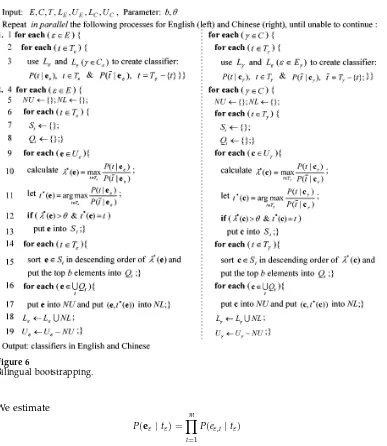
We perform bilingual bootstrapping as described in Figure 6. Note that we can, in principle, employ any kind of classifier here.

The figure explains the process for English (left-hand side); the process for Chinese (right-hand side) behaves similarly. At step 1, for each ambiguous wordε, we create binary classifiers for resolving its ambiguities (cf. lines 1–3). The main point here is that we use classified data from both languages to construct classifiers, as we describe in Section 3.2. For the example in Figure 3, we use bothLε(sentences P1 and P4) and Lγ, γ ∈ Cε (sentences Z1 and G1) to construct a classifier resolving ambiguities in Tε ={1, 2}. Note that not only P1 and P4, but also Z1 and G1, are related to {1, 2}. At step 2, for each wordε, we use its classifiers to select some unclassified instances fromUε, classify them, and add them toLε(cf. lines 4–19). We repeat the process until we cannot continue.

Lines 9–13 show that for each unclassified instance eε, we use the classifiers to classify it into the class (sense)tift’s posterior odds are the largest among the possible classes and are larger than a threshold θ. For each class t, we store the classified instances in St. Lines 14–15 show that for each class t, we choose only the top b

classified instances (in terms of the posterior odds), which are then stored inQt. Lines

16–17 show that we create the classified instances by combining the instances with their classification labels. We note that after line 17 we can also employ the one-sense-per-discourse heuristic.

3.2 An Implementation

Although we can in principle employ any kind of classifier in BB, we use here naive Bayes (or naive Bayesian ensemble). We also use the EM algorithm inclassified data transformationbetween languages. As will be made clear, this implementation of BB can naturally combine the features of naive Bayes (or naive Bayesian ensemble) and the features of EM. Hereafter, when we refer to BB, we mean this implementation of BB.

We explain the process for English (left-hand side of Figure 6); the process for Chinese (right-hand side of figure) behaves similarly. At step 1 in BB, we construct a naive Bayesian classifier as described in Figure 7. At step 2, for each instanceeε, we use the classifier to calculate

λ∗(eε) =max

tε∈Tε

P(tε|eε) P(¯tε|eε) =maxtε∈Tε

Figure 6

Bilingual bootstrapping.

We estimate

P(eε|tε) =

m

i=1

P(eε,i|tε)

We estimateP(eε|¯tε)similarly. We estimateP(eε|tε)by linearly combiningP(E)(eε|tε) estimated from English andP(C)_{(eε|tε)estimated from Chinese:}

P(eε|tε) = (1−α−β)P(E)(eε|tε) +αP(C)(eε|tε) +βP(U)(eε) (3)

where 0≤α≤1, 0≤β ≤1,α+β ≤1, andP(U)_{(eε)is a uniform distribution overE,}

which is used for avoiding zero probability. In this way, we estimate P(eε |tε)using information from not only English, but also Chinese.

We estimateP(E)_{(eε |tε)with maximum-likelihood estimation (MLE) usingLε as}

data. The estimation ofP(C)_{(eε|tε)proceeds as follows.}

For the sake of readability, we rewriteP(C)_{(eε |tε)asP(e| t). We define a}

finite-mixture model of the form P(c | t) = _e∈EP(c | e,t)P(e | t), and for a specificε we assume that the data in

estimate P(E)_{(eε|tε)with MLE usingLεas data;}

estimate P(C)_{(eε|tε)with EM algorithm usingLγ for eachγ∈Cεas data;}

calculateP(eε|tε)as a linear combination ofP(E)_{(eε|tε)and P}(C)_(eε|tε);

estimate P(tε)with MLE usingLε; calculateP(eε|¯_{tε)andP(¯tε)similarly.}

Figure 7

Creating a naive Bayesian classifier.

are generated independently from the model. We can therefore employ the expectation-maximization (EM) algorithm (Dempster, Laird, and Rubin 1977) to estimate the pa-rameters of the model, includingP(e|t). Note thateand crepresentcontext words.

Recall thatE is a set of words in English, C is a set of words in Chinese, and T is a set of senses. For a specific English word e,Ce ={c |(e,c) ∈T} represents the

Chinese words that are its possible translations. Initially, we set

P(c|e,t) =

  

1

|Ce|, ifc∈Ce

0, ifc∈Ce

P(e|t) = 1

|E|, e∈E

We next estimate the parameters by iteratively updating them, as described in Figure 8, until they converge. Heref(c,t)stands for the frequency of c in the instances which have senset. The context information in Chinesef(c,tε)is then “transformed” into the English versionP(C)_{(eε|tε)through the links inT.}

Figure 9 shows an example of estimatingP(eε|tε)with respect to thefactorysense (i.e., sense 1). We first use sentences such as P1 in Figure 3 to estimateP(E)_{(eε|tε)with}

MLE as described above. We next use sentences such as G1 to estimateP(C)_(eε|tε)as

described above. Specifically, with the frequency dataf(c,tε)and EM we can estimate P(C)_{(eε|tε). Finally, we linearly combineP}(E)_{(eε|tε)andP}(C)_{(eε|tε)to obtainP(eε|tε).} 3.3 Comparison of BB and MB

We note that monolingual bootstrapping is a special case of bilingual bootstrapping (consider the situation in whichα=0 in formula (3)).

BB can always perform better than MB. The asymmetric relationship between the ambiguous words in the two languages stands out as the key to the higher performance

E-step:P(e|c,t)← P(c|e,t)P(e|t)

e∈EP(c|e,t)P(e|t)

M-step:P(c|e,t)← f(c,t)P(e|c,t)

c∈Cf(c,t)P(e|c,t)

P(e|t)←

c∈Cf(c,t)P(e|c,t) c∈Cf(c,t) Figure 8

Figure 9

Parameter estimation.

Figure 10

Example application of BB.

of BB. By asymmetric relationship we mean the many-to-many mapping relationship between the words in the two languages, as shown in Figure 10.

Suppose that the classifier with respect to plant has two classes (denoted as A and B in Figure 10). Further suppose that the classifiers with respect togongchangand zhiwu in Chinese each have two classes (C and D) and (E and F), respectively. A and D are equivalent to one another (i.e., they represent the same sense), and so are B and E.

Assume that instances are classified after several iterations of BB as depicted in Figure 10. Here, circles denote the instances that are correctly classified and crosses denote the instances that are incorrectly classified.

Since A and D are equivalent to one another, we can transform the instances with D and use them to boost the performance of classification to A, because the misclassified instances (crosses) with D are those mistakenly classified from C, and they will not have much negative effect on classification to A, even though the translation from Chinese into English can introduce some noise. Similar explanations can be given for other classification decisions.

3.4 Relationship between BB and Co-training

We note that there are similarities between BB and co-training. Both BB and co-training execute two bootstrapping processes in parallel and make the two processes collabo-rate with one another in order to improve their performance. The two processes look at different types of information in data and exchange the information in learning. How-ever, there are also significant differences between BB and co-training. In co-training, the two processes use differentfeatures, whereas in BB, the two processes use different classes. In BB, although the features used by the two classifiers are transformed from one language into the other, they belong to the same space. In co-training, on the other hand, the features used by the two classifiers belong to two different spaces.

4. Experimental Results

We have conducted two experiments on English-Chinese translation disambiguation. In this section, we will first describe the experimental settings and then present the results. We will also discuss the results of several follow-on experiments.

4.1 Translation Disambiguation Using BB

Although it is possible to straightforwardly apply the algorithm of BB described in Section 3 to word translation disambiguation, here we use a variant of it better adapted to the task and for fairer comparison with existing technologies. The variant of BB we use has four modifications:

1. It actually employs naive Bayesian ensemble rather than naive Bayes, because naive Bayesian ensemble generally performs better than naive Bayes (Pedersen 2000).

2. It employs the one-sense-per-discourse heuristic. It turns out that in BB with one sense per discourse, there are two layers of bootstrapping. On the top level, bilingual bootstrapping is performed between the two languages, and on the second level, co-training is performed within each language. (Recall that MB with one sense per discourse can be viewed as co-training.)

3. It uses only classified data in English at the beginning. That is to say, it requires exactly the same human labeling efforts as MB does.

4. It individually resolves ambiguities on selected English words such as plantandinterest. (Note that the basic algorithm of BB performs

disambiguation on all the words in English and Chinese.) As a result, in the case ofplant, for example, the classifiers with respect togongchang andzhiwu make classification decisions only on D and E and not C and F (in Figure 10), because it is not necessary to make classification decisions on C and F. In particular, it calculatesλ∗(c)asλ∗(c) =P(c|t) and setsθ=0 in the right-hand side of step 2.

4.2 Translation Disambiguation Using MB

Table 1

Data descriptions in Experiment 1.

(QJOLVKZRUGV &KLQHVHZRUGV 6HQVHV 6HHGZRUGV UHDGLQHVVWRJLYHDWWHQWLRQ VKRZ PRQH\SDLGIRUWKHXVHRIPRQH\ UDWH DVKDUHLQFRPSDQ\RUEXVLQHVV KROG LQWHUHVW

DGYDQWDJHDGYDQFHPHQWRUIDYRU FRQIOLFW DWKLQIOH[LEOHREMHFW FXW

ZULWWHQRUVSRNHQWH[W ZULWH WHOHSKRQHFRQQHFWLRQ WHOHSKRQH IRUPDWLRQRISHRSOHRUWKLQJV ZDLW DQDUWLILFLDOGLYLVLRQ EHWZHHQ OLQH

SURGXFW SURGXFW

is, it employs a decision list as the classifier. This implementation is exactly the one proposed in Yarowsky (1995). (We will denote it as MB-D hereafter.) MB-B and MB-D can be viewed as the state-of-the-art methods for word translation disambiguation using bootstrapping.

4.3 Experiment 1: WSD Benchmark Data

We first applied BB, MB-B, and MB-D to translation disambiguation on the English words line and interest using a benchmark data set.5 _{The data set consists mainly}

of articles from the Wall Street Journal and is prepared for conducting word sense disambiguation (WSD) on the two words (e.g., Pedersen 2000).

We collected from the HIT dictionary6 _{the Chinese words that can be translations}

of the two English words; these are listed in Table 1. One sense of an English word links to one group of Chinese words. (For the word interest, we used only its four major senses, because the remaining two minor senses occur in only 3.3% of the data.) For each sense, we selected an English word that is strongly associated with the sense according to our own intuition (cf. Table 1). We refer to this word as a seed word. For example, for the sense of money paid for the use of money, we selected the word rate. We viewed the seed word as a classified “sentence,” following a similar proposal in Yarowsky (1995). In this way, for each sense we had a classified instance in English. As unclassified data in English, we collected sentences in news articles from a Web site (www.news.com), and as unclassified data in Chinese, we collected sentences in news articles from another Web site (news.cn.tom.com). Note that we need to use only the sentences containing the words in Table 1. We observed that the distribution of the senses in the unclassified data was balanced. As test data, we used the entire benchmark data set.

Table 2 shows the sizes of the data sets. Note that there are in general more unclassified sentences (and texts) in Chinese than in English, because one English word usually can link to several Chinese words (cf. Figure 5).

As the translation dictionary, we used the HIT dictionary, which contains about 76,000 Chinese words, 60,000 English words, and 118,000 senses (links). We then used the data to conduct translation disambiguation with BB, MB-B, and MB-D, as described in Sections 4.1 and Section 4.2.

5 http://www.d.umn.edu/∼tpederse/data.html.

Table 2

Data set sizes in Experiment 1.

Unclassified sentences (texts)

Words English Chinese Test sentences

interest 1,927 (1,072) 8,811 (2,704) 2,291 line 3,666 (1,570) 5,398 (2,894) 4,148

For both BB and MB-B, we used an ensemble of five naive Bayesian classifiers with window sizes of±1,±3,±5,±7, and±9 words, and we set the parametersβ,b, and θto 0.2, 15, and 1.5, respectively. The parameters were tuned on the basis of our preliminary experimental results on MB-B; they were not tuned, however, for BB. We set the BB-specific parameter α to 0.4, which meant that we weighted information from English and Chinese equally.

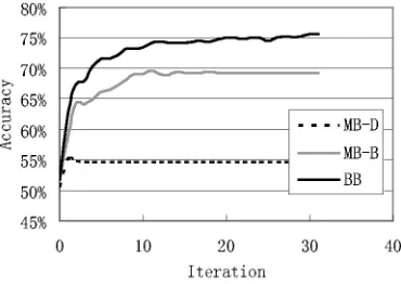
Table 3 shows the translation disambiguation accuracies of the three methods as well as that of a baseline method in which we always choose the most frequent sense. Figures 11 and 12 show the learning curves of MB-D, MB-B, and BB. Figure 13 shows the accuracies of BB with differentαvalues. From the results, we see that BBconsistently andsignificantlyoutperforms both MB-D and MB-B. The results from the sign test are statistically significant (p-value <0.001). (For the sign test method, see, for example, Yang and Liu [1999]).

Table 4 shows the results achieved by some existing supervisedlearning methods with respect to the benchmark data (cf. Pedersen 2000). Although BB is a method nearly equivalent to one based on unsupervised learning, it still performs favorably when compared with the supervised methods (note that since the experimental settings are different, the results cannot be directly compared).

4.4 Experiment 2: Yarowsky’s Words

We also conducted translation on seven of the twelve English words studied in Yarowsky (1995). Table 5 lists the words we used.

Table 3

Accuracies of disambiguation in Experiment 1.

Words Major (%) MB-D (%) MB-B (%) BB (%)

interest 54.6 54.7 69.3 75.5

line 53.5 55.6 54.1 62.7

Table 4

Accuracies of supervised methods.

interest (%) line (%)

Naive Bayesian ensemble 89 88

Naive Bayes 74 72

Decision tree 78 —

Neural network — 76

Figure 11

Learning curves withinterest.

Figure 12

Learning curves withline.

Figure 13

Table 5

Data set descriptions in Experiment 2.

(QJOLVKZRUGV &KLQHVHZRUGV 6HHGZRUGV

EDVV ILVKPXVLF

GUXJ WUHDWPHQWVPXJJOHU

GXW\ GLVFKDUJHH[SRUW

SDOP WUHHKDQG

SODQW LQGXVWU\OLIH

VSDFH YROXPHRXWHU

WDQN FRPEDWIXHO

Table 6

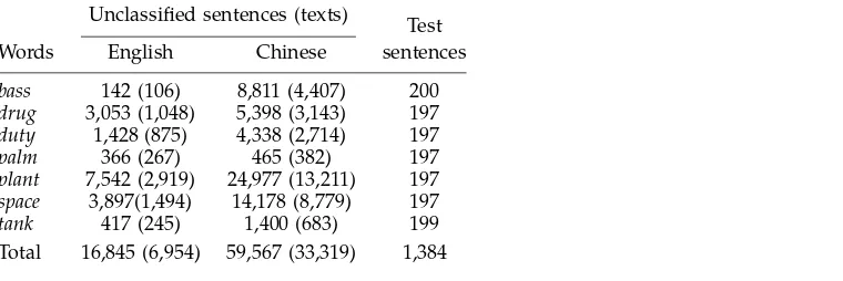
Data set sizes in Experiment 2.

Unclassified sentences (texts) _Test

Words English Chinese sentences

bass 142 (106) 8,811 (4,407) 200 drug 3,053 (1,048) 5,398 (3,143) 197 duty 1,428 (875) 4,338 (2,714) 197

palm 366 (267) 465 (382) 197

plant 7,542 (2,919) 24,977 (13,211) 197 space 3,897(1,494) 14,178 (8,779) 197 tank 417 (245) 1,400 (683) 199 Total 16,845 (6,954) 59,567 (33,319) 1,384

For each of the English words, we extracted about 200 sentences containing the word from the Encarta7 _{English corpus and hand-labeled those sentences using our}

own Chinese translations. We used the labeled sentences as test data and the unlabeled sentences as unclassified data in English. Table 6 shows the data set sizes. We also used the sentences in the Great Encyclopedia8 _{Chinese corpus as unclassified data in}

Chinese. We defined, for each sense, a seed word in English as a classified instance in English (cf. Table 5). We did not, however, conduct translation disambiguation on the wordscrane, sake, poach, axes, andmotion, because the first four words do not frequently occur in the Encarta corpus, and the accuracy of choosing the major translation for the last word already exceeds 98%.

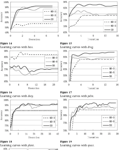
We next applied BB, MB-B, and MB-D to word translation disambiguation. The parameter settings were the same as those in Experiment 1. Table 7 shows the dis-ambiguation accuracies, and Figures 14–20 show the learning curves for the seven words.

From the results, we see again that BB significantly outperforms MB-D and MB-B. Note that the results of MB-D here cannot be directly compared with those in Yarowsky (1995), because the data used are different. Naive Bayesian ensemble did not perform well on the wordduty, causing the accuracies of both MB-B and BB to deteriorate.

Figure 14 Figure 15

Learning curves withbass. Learning curves withdrug.

Figure 16 Figure 17

Learning curves withduty. Learning curves withpalm.

Figure 18 Figure 19

Learning curves withplant. Learning curves withspace.

Figure 20

Table 7

Accuracies of disambiguation in Experiment 2.

Words Major (%) MB-D (%) MB-B (%) BB (%)

bass 61.0 57.0 89.0 92.0

drug 77.7 78.7 79.7 86.8

duty 86.3 86.8 72.0 75.1

palm 82.2 80.7 83.3 92.4

plant 71.6 89.3 95.4 95.9

space 64.5 83.3 84.3 87.8

tank 60.3 76.4 76.9 84.4

Total 71.9 78.8 82.9 87.8

Table 8

Top words forinterest ratesense ofinterest.

MB-B BB

payment saving

cut payment

earn benchmark

short whose

short-term base yield prefer

u.s. fixed

margin debt

benchmark annual regard dividend

4.5 Discussion

We investigated the reason for BB’s outperforming MB and found that the explanation in Section 3.3 appears to be valid according to the following observations.

1. In a naive Bayesian classifier, words with large values of likelihood ratio P_P(₍e|t_e|¯_t))

will have strong influences on classification. We collected the words having the largest likelihood ratio with respect to each sense tin both BB and MB-B and found that BB obviously has more “relevant words” than MB-B. Here words relevant to a particular sense refer to the words that are strongly indicative of that sense according to human judgments.

Table 8 shows the top 10 words in terms of likelihood ratio with respect to the interest rate sense in both BB and MB-B. The relevant words are italicized. Figure 21 shows the numbers of relevant words with respect to the four senses ofinterestin BB and MB-B.

2. From Figure 13, we see that the performance of BB remains high or gets higher even whenαbecomes larger than 0.4 (recall thatβwas fixed at 0.2). This result strongly indicates that the information from Chinese has positive effects.

Figure 21

Number of relevant words.

Figure 22

When more unclassified data available.

data increases. Figure 22 plots again the results of BB as well as those of a method referred to as MB-C. In MB-C, we linearly combined two MB-B classifiers constructed with two different unclassified data sets, and we found that although the accuracies are improved in MB-C, they are still much lower than those of BB.

4. We have noticed that a key to BB’s performance is the asymmetric relationship between the classes in the two languages. Therefore, we tested the performance of MB and BB when the classes in the two languages are symmetric (i.e., one-to-one mapping).

We performed two experiments on text classification in which the categories were finance and industry, and finance and trade, respectively. We collected Chinese texts from the People’s Dailyin 1998 that had already been assigned class labels. We used half of them as unclassified training data in Chinese and the remaining as test data in Chinese. We also collected English texts from theWall Street Journal. We used them as unlabeled training data in English. We used the class names (i.e.,finance, industry, and trade, as seed data (classified data)). Table 9 shows the accuracies of text classification. From the results we see that when the classes are symmetric, BB cannot outperform MB.

Table 9

Accuracy of text classification.

Classes MB-B (%) BB (%)

Finance and industry 93.2 92.9 Finance and trade 78.4 78.6

Table 10

Accuracy of disambiguation.

MB-D (%) MB-B (%) BB (%)

With one sense per discourse 54.7 69.3 75.5 Without one sense per discourse 54.6 66.4 71.6

5. Conclusion

We have addressed here the problem of classification across two languages. Specifically we have considered the problem of bootstrapping. We find that when the task is word translation disambiguation between two languages, we can use the asymmetric rela-tionship between the ambiguous words in the two languages to significantly boost the performance of bootstrapping. We refer to this approach as bilingual bootstrapping. We have developed a method for implementing this bootstrapping approach that nat-urally combines the use of naive Bayes and the EM algorithm. Future work includes a theoretical analysis of bilingual bootstrapping (generalization error of BB, relationship between BB and co-training, etc.) and extensions of bilingual bootstrapping to more complicated machine translation tasks.

Acknowledgments

We thank Ming Zhou, Ashley Chang and Yao Meng for their valuable comments and suggestions on an early draft of this article. We acknowledge the four anonymous reviewers of this article for their valuable comments and criticisms. We thank Michael Holmes, Mark Petersen, Kevin Knight, and Bob Moore for their checking of the English of this article. A previous version of this article appeared inProceedings of the Fortieth Annual Meeting of the Association for

Computational Linguistics.

References

Banko, Michele, and Eric Brill. 2001. Scaling to very very large corpora for natural language disambiguation. InProceedings of the 39th Annual Meeting of the Association for Computational Linguistics, pages 26–33, Toulouse, France.

Blum, Avrim, and Tom M. Mitchell. 1998. Combining labeled and unlabeled data with co-training. InProceedings of the 11th Annual Conference on Computational

Learning Theory, pages 92–100, Madison, WI.

Brown, Peter F., Stephen A. Della Pietra, Vincent J. Della Pietra, and Robert L. Mercer. 1991. Word sense disambiguation using statistical methods. InProceedings of the 29th Annual Meeting of the Association for Computational Linguistics, pages 264–270, University of California, Berkeley. Bruce, Rebecca, and Janyce Weibe. 1994.

Word-sense disambiguation using

decomposable models. InProceedings of the 32nd Annual Meeting of the Association for Computational Linguistics, pages 139–146, New Mexico State University, Las Cruces. Collins, Michael, and Yoram Singer. 1999.

Unsupervised models for named entity classification. InProceedings of the 1999 Joint SIGDAT Conference on Empirical Methods in Natural Language Processing and Very Large Corpora, University of

Maryland, College Park.

Dempster, A. P., N. M. Laird, and D. B. Rubin. 1977. Maximum likelihood from incomplete data via the EM algorithm. Journal of the Royal Statistical Society B, 39:1–38.

Escudero, Gerard, Lluis Marquez, and German Rigau. 2000. Boosting applied to word sense disambiguation. InProceedings of the 12th European Conference on Machine Learning, pages 129–141, Barcelona. Gale, William, Kenneth Church, and David

Yarowsky. 1992a. A method for disambiguating word senses in a large corpus.Computers and Humanities, 26:415–439.

Gale, William, Kenneth Church, and David Yarowsky. 1992b. One sense per discourse. InProceedings of DARPA Speech and Natural Language Workshop, pages 233–237, Harriman, NY.

Golding, Andrew R., and Dan Roth. 1999. A Winnow-based approach to

context-sensitive spelling correction. Machine Learning, 34:107–130.

Kikui, Genichiro. 1999. Resolving translation ambiguity using non-parallel bilingual corpora. InProceedings of ACL ’99 Workshop on Unsupervised Learning in Natural Language Processing, University of Maryland, College Park.

Koehn, Philipp, and Kevin Knight. 2000. Estimating word translation probabilities from unrelated monolingual corpora using the EM algorithm. InProceedings of the 17th National Conference on Artificial Intelligence, pages 711–715, Austin, TX.

Li, Hang, and Kenji Yamanishi. 2002. Text classification using ESC-based stochastic decision lists.Information Processing and Management, 38:343–361.

Lin, Dekang. 1997. Using syntactic dependency as local context to resolve word sense ambiguity. InProceedings of the 35th Annual Meeting of the Association for Computational Linguistics, pages 64–71, Universidad Nacional de Educaci ´on a Distancia (UNED), Madrid.

Mangu, Lidia, and Eric Brill. 1997. Automatic rule acquisition for spelling correction. InProceedings of the 14th International Conference on Machine Learning, pages 187–194, Nashville, TN.

Mihalcea, Rada, and Dan I. Moldovan. 1999. A method for word sense disambiguation of unrestricted text. InProceedings of the 37th Annual Meeting of the Association for Computational Linguistics, pages 152–158, University of Maryland, College Park. Ng, Hwee Tou, and Hian Beng Lee. 1996.

Integrating multiple knowledge sources to disambiguate word sense: An

exemplar-based approach. InProceedings of the 34th Annual Meeting of the Association for

Computational Linguistics, pages 40–47, University of California, Santa Cruz. Nigam, Kamal, Andrew McCallum,

Sebastian Thrun, and Tom M. Mitchell. 2000. Text classification from labeled and unlabeled documents using EM.Machine Learning, 39(2–3):103–134.

Nigam, Kamal, and Rayid Ghani. 2000. Analyzing the effectiveness and

applicability of co-training. InProceedings of the 9th International Conference on Information and Knowledge Management, pages 86–93, McLean, VA.

Pedersen, Ted. 2000. A simple approach to building ensembles of naive Bayesian classifiers for word sense disambiguation. InProceedings of the First Meeting of the North American Chapter of the Association for Computational Linguistics, Seattle.

Pedersen, Ted, and Rebecca Bruce. 1997. Distinguishing word senses in untagged text. InProceedings of the Second Conference on Empirical Methods in Natural Language Processing, pages 197–207, Providence, RI. Pierce, David, and Claire Cardie. 2001.

Limitations of co-training for natural language learning from large datasets. In Proceedings of the 2001 Conference on Empirical Methods in Natural Language Processing, Carnegie Mellon University, Pittsburgh.

Schutze, Hinrich. 1998. Automatic word sense discrimination.Computational Linguistics, 24(1):97–124.

Towell, Geoffrey, and Ellen M. Voorhees. 1998. Disambiguating highly ambiguous words.Computational Linguistics,

24(1):125–146.

Yang, Yiming, and Xin Liu. 1999. A re-examination of text categorization methods. InProceedings of the 22nd Annual International ACM SIGIR Conference on Research and Development in Information Retrieval, pages 42–49, Berkeley, CA. Yarowsky, David. 1994. Decision lists for

lexical ambiguity resolution: Application to accent restoration in Spanish and French. InProceedings of the 32nd Annual Meeting of the Association for Computational Linguistics, pages 88–95, New Mexico State University, Las Cruces.

Yarowsky, David. 1995. Unsupervised word sense disambiguation rivaling supervised methods. InProceedings of the 33rd Annual Meeting of the Association for Computational Linguistics, pages 189–196.