A Statistical Parsing Framework for Sentiment Classification

Sentiment Classification

Li Dong

∗,∗∗ Beihang University

Furu Wei

†,‡ Microsoft Research

Shujie Liu

† Microsoft Research

Ming Zhou

† Microsoft Research

Ke Xu

∗

Beihang University

We present a statistical parsing framework for sentence-level sentiment classification in this article. Unlike previous works that use syntactic parsing results for sentiment analysis, we develop a statistical parser to directly analyze the sentiment structure of a sentence. We show that complicated phenomena in sentiment analysis (e.g., negation, intensification, and contrast) can be handled the same way as simple and straightforward sentiment expressions in a unified and probabilistic way. We formulate the sentiment grammar upon Context-Free Grammars (CFGs), and provide a formal description of the sentiment parsing framework. We develop the parsing model to obtain possible sentiment parse trees for a sentence, from which the polarity model is proposed to derive the sentiment strength and polarity, and the ranking model is dedicated to selecting the best sentiment tree. We train the parser directly from examples of sentences annotated only with sentiment polarity labels but without any syntactic annotations or polarity annotations of constituents within sentences. Therefore we can obtain training data easily. In particular, we train a sentiment parser, s.parser, from a large amount of review sentences with users’ ratings as rough sentiment polarity labels. Extensive experiments on existing benchmark data sets show significant improvements over baseline sentiment classification approaches.

∗State Key Laboratory of Software Development Environment, Beihang University, XueYuan Road No.37, HaiDian District, Beijing, P.R. China 100191. E-mail:[email protected]; [email protected].

∗∗Contribution during internship at Microsoft Research.

†Natural Language Computing Group, Microsoft Research Asia, Building 2, No. 5 Danling Street, Haidian District, Beijing, P.R. China 100080. E-mail:{fuwei, shujliu, mingzhou}@microsoft.com.

‡Corresponding author.

Submission received: 10 December 2013; revised version received: 26 July 2014; accepted for publication: 28 January 2015.

1. Introduction

Sentiment analysis (Pang and Lee 2008; Liu 2012) has received much attention from both research and industry communities in recent years. Sentiment classification, which identifies sentiment polarity (positive or negative) from text (sentence or document), has been the most extensively studied task in sentiment analysis. Until now, there have been two mainstream approaches for sentiment classification. The lexicon-based approach (Turney 2002; Taboada et al. 2011) aims to aggregate the sentiment polarity of a sentence from the polarity of words or phrases found in the sentence, and the learning-based approach (Pang, Lee, and Vaithyanathan 2002) treats sentiment polarity identification as a special text classification task and focuses on building classifiers from a set of sentences (or documents) annotated with their corresponding sentiment polarity.

The lexicon-based sentiment classification approach is simple and interpretable, but suffers from scalability and is inevitably limited by sentiment lexicons that are commonly created manually by experts. It has been widely recognized that sentiment expressions are colloquial and evolve over time very frequently. Taking tweets from Twitter1 and movie reviews on IMDb2 as examples, people use very casual language as well as informal and new vocabulary to comment on general topics and movies. In practice, it is not feasible to create and maintain sentiment lexicons to capture sentiment expressions with high coverage. On the other hand, the learning-based approach relies on large annotated samples to overcome the vocabulary coverage and deals with varia-tions of words in sentences. Human ratings in reviews (Maas et al. 2011) and emoticons in tweets (Davidov, Tsur, and Rappoport 2010; Zhao et al. 2012) are extensively used to collect a large number of training corpora to train the sentiment classifier. However, it is usually not easy to design effective features to build the classifier. Among others, unigrams have been reported as the most effective features (Pang, Lee, and Vaithyanathan 2002) in sentiment classification.

Handling complicated expressions delivering people’s opinions is one of the most challenging problems in sentiment analysis. Compositionalities such as negation, inten-sification, contrast, and their combinations are typical cases. We show some concrete examples here:

(1) The movie is notgood. [negation] (2) The movie is verygood. [intensification]

(3) The movie is notfunnyat all. [negation + intensification] (4) The movie isjust so so, but i stilllikeit. [contrast]

(5) The movie is not verygood, but i stilllikeit. [negation + intensification + contrast]

The negation expressions, intensification modifiers, and the contrastive conjunction can change the polarity (Examples (1), (3), (4), (5)), strength (Examples (2), (3), (5)), or both (Examples (3), (5)) of the sentiment of the sentences. We do not need any detailed explanations here as they can be commonly found and easily understood in people’s

1http://twitter.com.

daily lives. Existing works to address these issues usually rely on syntactic parsing results either used as features (Choi and Cardie 2008; Moilanen, Pulman, and Zhang 2010) in learning-based methods or hand-crafted rules (Moilanen and Pulman 2007; Jia, Yu, and Meng 2009; Klenner, Petrakis, and Fahrni 2009; Liu and Seneff 2009) in lexicon-based methods. However, even with the difficulty and feasibility of deriving the senti-ment structure from syntactic parsing results put aside, it is an even more challenging task to generate stable and reliable parsing results for text that is ungrammatical in nature and has a high ratio of out-of-vocabulary words. The accuracy of the linguistic parsers trained on standard data sets (e.g., the Penn Treebank [Marcus, Marcinkiewicz, and Santorini 1993]) drops dramatically on user-generated-content (reviews, tweets, etc.), which is actually the prime focus of sentiment analysis algorithms. The error, unfortunately, will propagate downstream in the process of sentiment analysis methods building upon parsing results.

We therefore propose directly analyzing the sentiment structure of a sentence. The nested structure of sentiment expressions can be naturally modeled in a similar fashion as statistical syntactic parsing, which aims to find the linguistic structure of a sentence. This idea creates many opportunities for developing sentiment classifiers from a new perspective. The most challenging problem and barrier in building a statistical sentiment parser lies in the acquisition of training data. Ideally, we need examples of sentences annotated with polarity for the whole sentence as well as sentiment tags for constituents within a sentence, as with the Penn TreeBank for training traditional linguistic parsers. However, this is not practical as the annotations will be inevitably time-consuming and require laborious human efforts. Therefore, it is better to learn the sentiment parser only utilizing examples annotated with the polarity label of the whole sentence. For example, we can collect a huge number of publicly available reviews and rating scores on the Web. People may usethe movie is gud(“gud” is a popular informal expression of “good”) to express a positive opinion towards a movie, andnot a fanto express a negative opinion. Also, we can find review sentences such as The movie is gud, but I am still not a fanto indicate a negative opinion. We can then use these two fragments and the overall negative opinion of the sentence to deduce sentiment rules automatically from data. These sentiment fragments and rules can be used to analyze the sentiment structure for new sentences.

The major contributions of the work presented in this article are as follows.

r

_{We propose a statistical parsing framework for sentiment analysis that is}

capable of analyzing the sentiment structure for a sentence. This

framework can naturally handle compositionality in a probabilistic way. It can be trained from sentences annotated with only sentiment polarity but without any syntactic annotations or polarity annotations of constituents within sentences.

r

_{We present the parsing model, polarity model, and ranking model in the}

proposed framework, which are formulated and can be improved

independently. It provides a principled and flexible approach to sentiment classification.

r

_{We implement the statistical sentiment parsing framework, and conduct}

experiments on several benchmark data sets. The experimental results show that the proposed framework and algorithm can significantly outperform baseline methods.

The remainder of this article is organized as follows. We introduce related work in Section 2. We present the statistical sentiment parsing framework, including the parsing model, polarity model, and ranking model, in Section 3. Learning methods for our model are explained in Section 4. Experimental results are reported in Section 5. We conclude this article with future work in Section 6.

2. Related Work

In this section, we give a brief introduction to related work about sentiment classi-fication (Section 2.1) and parsing (Section 2.2). We tackle the sentiment classiclassi-fication problem in a parsing manner, which is a significant departure from most previous research.

2.1 Sentiment Classification

Sentiment classification has been extensively studied in the past few years. In terms of text granularity, existing works can be divided into phrase-level, sentence-level, or document-level sentiment classification. We focus on sentence-level sentiment classifi-cation in this article. Regardless of what granularity the task is performed on, existing approaches deriving sentiment polarity from text fall into two major categories, namely, lexicon-based and learning-based approaches.

any labeled samples. But they suffer from coverage and domain adaption problems. Moreover, lexicons are often built and used without considering the context (Wilson, Wiebe, and Hoffmann 2009). Also, hand-crafted rules are often matched heuristically.

The sentiment dictionaries used for lexicon-based sentiment analysis can be cre-ated manually, or automatically using seed words to expand the list of words. Kamps et al. (2004) and Williams and Anand (2009) used various lexical relations (such as synonym and antonym relations) in WordNet to expend a set of seed words. Some other methods learn lexicons from data directly. Hatzivassiloglou and McKeown (1997) used a log-linear regression model with conjunction constraints to predict whether conjoined adjectives have similar or different polarities. Combining conjunction constraints across many adjectives, a clustering algorithm separated the adjectives into groups of different polarity. Finally, adjectives were labeled as positive or negative. Velikovich et al. (2010) constructed a term similarity graph using the cosine similarity of context vectors. They performed graph propagation from seeds on the graph, obtaining polarity words and phrases. Takamura, Inui, and Okumura (2005) regarded the polarity of words as spins of electrons, using the mean field approximation to compute the approximate probability function of the system instead of the intractable actual probability function. Kanayama and Nasukawa (2006) used tendencies for similar polarities to appear successively in contexts. They defined density and precision of coherency to filter neutral phrases and uncertain candidates. Choi and Cardie (2009a) and Lu et al. (2011) transformed the lexicon learning to an optimization problem, and used integer linear programming to solve it. Kaji and Kitsuregawa (2007) defined theχ2-based polarity value and PMI-based polarity value as a polarity strength to filter neutral phrases. de Marneffe, Manning, and Potts (2010) utilized review data to define polarity strength as the expected rating value. Mudinas, Zhang, and Levene (2012) used word count as a feature template and trained a classifier using Support Vector Machines with linear kernel. They then re-garded the weights as polarity strengths. Krestel and Siersdorfer (2013) generated topic-dependent lexicons from review articles by incorporating topic and rating probabilities and defined the polarity strength based on the results. In this article, the lexical relations defined in WordNet are not used because of its coverage. Furthermore, most of these methods define different criteria to propagate polarity information of seeds, or use optimization algorithms and sentence-level sentiment labels to learn polarity strength values. Their goal is to balance the precision and recall of learned lexicons. We also learn the polarity strength values of phrases from data. However, our primary objective is to obtain correct sentence-level polarity labels, and use them to form the sentiment grammar.

extract frequent subsequences and dependency subtrees, and used them as features of SVM. McDonald et al. (2007) investigated a global structured model for jointly classifying polarity at different levels of granularity. This model allowed classification decisions from one level in the text to influence decisions at another. Yessenalina, Yue, and Cardie (2010) used sentence-level latent variables to improve document-level prediction. T¨ackstr ¨om and McDonald (2011a) presented a latent variable model for only using document-level annotations to learn sentence-level sentiment labels, and T¨ackstr ¨om and McDonald (2011b) improved it by using a semi-supervised latent vari-able model to utilize manually crafted sentence labels. Agarwal et al. (2011) and Tu et al. (2012) explored part-of-speech tag features and tree-kernel. Wang and Manning (2012) used SVM built over Na¨ıve Bayes log-count ratios as feature values to classify polarity. They showed that SVM was better at full-length reviews, and Multinomial Na¨ıve Bayes was better at short-length reviews. Liu, Agam, and Grossman (2012) proposed a set of heuristic rules based on dependency structure to detect negations and sentiment-bearing expressions. Most of these methods are built on bag-of-words features, and sentiment compositions are handled by manually crafted rules. In contrast to these models, we derive polarity labels from tree structures parsed by the sentiment grammar. There have been several attempts to assume that the problem of sentiment analy-sis is compositional. Sentiment classification can be solved by deriving the sentiment of a complex constituent (sentence) from the sentiment of small units (words and phrases) (Moilanen and Pulman 2007; Klenner, Petrakis, and Fahrni 2009; Choi and Cardie 2010; Nakagawa, Inui, and Kurohashi 2010). Moilanen and Pulman (2007) pro-posed using delicate written linguistic patterns as heuristic decision rules when com-puting the sentiment from individual words to phrases and finally to the sentence. The manually compiled rules were powerful enough to discriminate between the different sentiments ineffective remedies(positive) /effective torture(negative), and intoo colorful

compositions by defining sentiment grammar and borrowing some techniques in the parsing research field. Moreover, our method uses symbolic representations instead of vector spaces.

2.2 Syntactic Parsing and Semantic Parsing

The work presented in this article is close to traditional statistical parsing, as we borrow some algorithms to build the sentiment parser. Syntactic parsers are learned from the Treebank corpora, and find the most likely parse tree with the largest probability. In this article, we borrow some well-known techniques from syntactic parsing methods (Charniak 1997; Charniak and Johnson 2005; McDonald, Crammer, and Pereira 2005; K ¨ubler, McDonald, and Nivre 2009), such as the CYK algorithm and Context-Free Grammar. These techniques are used to build the sentiment grammar and parsing model. They provide a natural way of defining the structure of sentiment trees and parse sentences to trees. The key difference lies in that our task is to calculate the polarity label of a sentence, instead of obtaining the parse tree. We only have sentence-polarity pairs as our training instances instead of annotated tree structures. Moreover, in the decoding process, our goal is to compute correct polarity labels by representing sentences as latent sentiment trees. Recently, Hall, Durrett, and Klein (2014) developed a discriminative constituency parser using rich surface features, adapting it to sentiment analysis. Besides extracting unigrams and bigrams as features, they learned interactions between tags and words located at the beginning or the end of spans. However, their method relies on phrase-level polarity annotations.

3. Statistical Sentiment Parsing

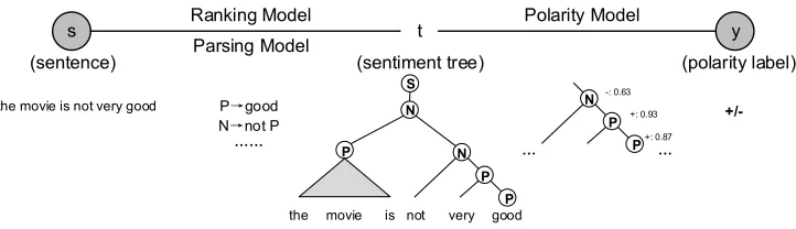
We present the statistical parsing framework for sentence-level sentiment classification in this section. The underlying idea is to model sentiment classification as a statisti-cal parsing process. Figure 1 shows the overview of the statististatisti-cal sentiment parsing framework. There are three major components. The input sentence s is transformed into and represented by sentiment trees derived from the parsing model (Section 3.2), using the sentiment grammar defined in Section 3.1. Trees are scored by the ranking model in Section 3.3. The sentiment tree with the highest ranking score is treated as the best derivation fors. Furthermore, the polarity model (Section 3.4) is used to compute polarity values for the sentiment trees.

Notably, the sentiment treestare unobserved during training. We can only observe the sentencesand its polarity labelyin training data. In other words, we train the model directly from the examples of sentences annotated only with sentiment polarity labels but without any syntactic annotations or polarity annotations of the constituents within sentences. To be specific, we first learn the sentiment grammar and the polarity model from data as described in Section 4.2. Then, given the sentence and polarity label pairs

s,y, we search the latent sentiment treestand estimate the parameters of the ranking model as detailed in Section 4.1.

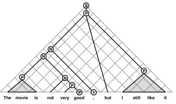
To better illustrate the whole process, we describe the sentiment parsing procedure using an example sentence,The movie is not very good, but i still like it. The sentiment polarity label of the above sentence is “positive.” There is negation, intensification, and contrast in this example, which are difficult to capture using bag-of-words classification methods. This sentence is a complex case that demonstrates the capability of the pro-posed statistical sentiment parsing framework, which motivates the work in this article. The statistical sentiment parsing algorithm may generate a number of sentiment trees for the input sentence. Figure 2 shows the best sentiment parse tree. It shows that the statistical sentiment parsing framework can deal with the compositionality of sentiment in a natural way. In Table 1, we list the sentiment rules used during the parsing process. We show the generation process of the sentiment parse tree from the bottom–up and the calculation of sentiment strength and polarity for every text span in the parsing process.

s t y

(sentence) Parsing Model (sentiment tree) (polarity label) Ranking Model Polarity Model

the movie is not very good P→good

+/-N→not P

…… _P

P P N

N S

the movie is not very good

P P N

… …

[image:8.486.51.412.502.606.2]

+: 0.87 +: 0.93 -: 0.63

Figure 1

The movie is not very good , but I still like it P

P

P ε

P P

N N

N

[image:9.486.54.351.67.242.2]

S

Figure 2

Sentiment structure for the sentenceThe movie is not very good, but i still like it. The rules used in the derivation process include{P→the movie is;P→good;P→i still like it;P→veryP; N→notP;N→PN;N→NE;E→,;P→NbutP;S→P}.

In the following sections, we first provide a formal description of the sentiment grammar in Section 3.1. We then present the details of the parsing model in Section 3.2, the ranking model in Section 3.3, and the polarity model in Section 3.4.

3.1 Sentiment Grammar

We develop the sentiment grammar upon CFG (Context-Free Grammar) (Chomsky 1956). Let G=<V,Σ,S,R> denote a CFG, where V is a finite set of non-terminals,

Σis a finite set of terminals (disjointed from V),S∈V is the start symbol, and R is a set of rewrite rules (or production rules) of the formA→c where A∈V and c∈

(V∪Σ)∗. We useG_s=<Vs,Σs,S,Rs>to denote the sentiment grammar in this article.

Table 1

Parsing process for the sentenceThe movie is not very good, but i still like it. [i,Y,j] represents the text spanning fromitojis derived to symbolY.NandPare non-terminals in the sentiment grammar, andNandPrepresent polarities of sentiment.

Span Rule Strength Polarity

[0,P, 3]: the movie is P→the movie is 0.52 P

[5,P, 6]: good P→good 0.87 P

[6,E, 7]: , E→, -

-[8,P, 11]: i still like it P→i still like it 0.85 P

[4,P, 6]: very good P→veryP 0.93 P

[3,N, 6]: not very good N→notP 0.63 N

[0,N, 6]: the movie is not very good N→PN 0.60 N

[0,N, 7]: the movie is not very good, N→NE 0.60 N

[0,P, 11]: the movie is not very good, but i still like it P→NbutP 0.76 P

[image:9.486.66.436.538.662.2]

The non-terminal set is denoted as Vs ={N,P,S,E}, where S is the start symbol, the

non-terminalNrepresents the negative polarity, and the non-terminalPrepresents the positive polarity. The rules inRsare divided into the following six categories:

r

_{Dictionary rules:X}→wk

0, whereX∈ {N,P},wk0=w0. . .wk−1, and

wk₀∈Σ+_s . These rules can be regarded as the sentiment dictionary used in traditional approaches. They are basic sentiment units assigned with polarity probabilities. For instance,P→good is a dictionary rule.

r

_{Combination rules:X}→c, wherec∈(Vs∪Σs)+, and two successive

non-terminals are not allowed. There is at least one terminal inc. These rules combine terminals and non-terminals, such asN→notP, andP→NbutP. They are used to handle negation, intensification, and contrast in sentiment analysis. The number of non-terminals in a combination rule is restricted to one and two.

r

_{Glue rules:X}→X1X2, whereX,X1,X2 ∈ {N,P}. These rules combine two text spans that are derived intoX1andX2, respectively.

r

_{OOV rules:}E →wk₀, wherewk₀ ∈Σ+. We use these rules to handle

Out-Of-Vocabulary (OOV) text spans whose polarity probabilities are not learned from data.

r

_{Auxiliary rules:X}→EX1,X→X1E, whereX,X1 ∈ {N,P}. These rules combine a text span with polarity and an OOV text span.

r

_{Start rules:S}→Y, whereY∈ {N,P,E}. The derivations begin withS, andS

can be derived toN,P, andE.

Here, X represents the non-terminals N or P. The dictionary rules and combi-nations rules are automatically extracted from the data. We will describe the details in Section 4.2. By applying these rules, we can derive the polarity label of a sen-tence from the bottom–up. The glue rules are used to combine polarity informa-tion of two text spans together, and it treats the combined parts as independent. In order to tackle the OOV problem, we treat a text span that consists of OOV words as empty text span, and derive them toE. The OOV text spans are combined with other text spans without considering their sentiment information. Finally, each sentence is derived to the symbol S using the start rules that are the beginnings of derivations. We can use the sentiment grammar to compactly describe the derivation process of a sentence.

3.2 Parsing Model

We present the formal description of the statistical sentiment parsing model following deductive proof systems (Shieber, Schabes, and Pereira 1995; Goodman 1999) as used in traditional syntactic parsing. For a concrete example,

(A→BC) [i,B,k] [k,C,j]

which represents if we have the ruleA→BCand B⇒∗ wk_i and C⇒∗ w_kj (⇒∗ is used to represent the reflexive and transitive closure of immediate derivation), then we can obtainA⇒∗ w_ij. By adding a unary rule

(A→wj_i)

[i,A,j] (7)

with the binary rule in Equation (6), we can express the standard CYK algorithm for CFG in Chomsky Normal Form (CNF). And the goal is [0,S,n], in whichSis the start symbol andnis the length of the input sentence. In the given CYK example, the term in deductive rules can be one of the following two forms:

r

_{[i,X,j] is anitemrepresenting a subtree rooted inXspanning fromitoj, or}

r

_(X→γ) is arulein the grammar.

Generally, we represent the form of an inference rule as:

(r) H1 . . . HK

[i,X,j] (8)

where, if all the termsrandHkare true, then we can infer [i,X,j] as true. Here,rdenotes

a sentiment rule, andHkdenotes an item. When we refer to both rules and items, we

employ the wordterms.

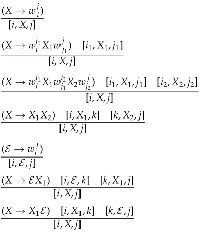
Theoretically, we can convert the sentiment rules to CNF versions, and then use the CYK algorithm to conduct parsing. Because the maximum number of non-terminal symbols in a rule is already restricted to two, we formulate the statistical sentiment parsing based on a customized CYK algorithm that is similar to the work of Chiang (2007). Let X,X1,X2 represent the non-terminals N or P; the inference rules for the statistical sentiment parsing are summarized in Figure 3.

3.3 Ranking Model

The parsing model generates many candidate parse treesT(s) for a sentence s. The goal of the ranking model is to score and rank these parse trees. The sentiment tree with the highest score is treated as the best representation for sentences. We extract a feature vectorφ(s,t)∈Rd for the specific sentence-tree pair (s,t), wheret∈T(s) is the parse tree. Letψ∈Rd be the parameter vector for the features. We use the log-linear model to calculate a probabilityp(t|s;T,ψ) for each parse treet∈T(s). The probabilities indicate how likely the trees are to produce correct predictions. Given the sentences

and parametersψ, the log-linear model defines a conditional probability:

p(t|s;T,ψ)=exp{φ(s,t)Tψ−A(ψ;s,T)} (9)

A(ψ;s,T)=log X

t∈T(s)

(X→wj_i) [i,X,j]

(X→wi1_iX1wjj1) [i1,X1,j1] [i,X,j]

(X→wi1_iX1wi2j1X2wj2j) [i1,X1,j1] [i2,X2,j2] [i,X,j]

(X→X1X2) [i,X1,k] [k,X2,j] [i,X,j]

(E→w_ij) [i,E,j]

(X→EX1) [i,E,k] [k,X1,j] [i,X,j]

(X→X1E) [i,X1,k] [k,E,j] [i,X,j]

[image:12.486.49.243.74.304.2]

whereX,X1,X2representNorP.

Figure 3

Inference rules for the basic parsing model.

where A(ψ;s,T) is the log-partition function with respect to T(s). The log-linear model is a discriminative model, and it is widely used in natural language pro-cessing. We can useφ(s,t)Tψas the score of the parse tree without normalization in the decoding process, becausep(t|s;T,ψ)∝φ(s,t)Tψ, and this will not change the ranking order.

3.4 Polarity Model

The goal of the polarity model is to model the calculation of sentiment strength and polarity of a text span from its subspans in the parsing process. It is specified in terms of the rules used in the parsing process. We expand the notations in the inference rule (8) to incorporate the polarity model. The new form of inference rule is:

(r) H1Φ1 . . . HKΦK

[i,X,j]Φ (11)

in whichr,H1,. . .,HKare the terms described in Section 3.2. Every itemHkis assigned

polarity strengthΦ_k: (

P(N|wjk ik)

P(P|w_ikjk) for text spanw

jk

ik. For the item [i,X,j], the polarity

modelΦ(r,Φ₁,. . .,ΦK) is defined as a function that takes the rulerand polarity strength

The polarity strength obtained by the polarity model should satisfy two con-straints. First, the values calculated by the polarity model are non-negative, that is,

P(X|wj_i)≥0,P(X|wj_i)≥0. Second, the positive and negative polarity values are

normal-ized to 1, namely,P(X|wj_i)+P(X|wj_i)=1. Notably,X =

(

P, X =N

N, X =P is the opposite

polarity ofX.

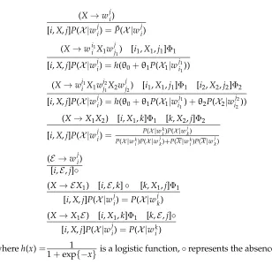
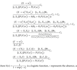
The inference rules with the polarity model are formally defined in Figure 4. In the following part, we define the polarity model for the different types of rules. If the rule is a dictionary ruleX→wj_i, its sentiment strength is obtained as:

Φ:

(

P(X|wj_i)=P˜(X|wj_i)

P(X|wj_i)=P˜(X|wj_i) (12)

whereX ∈ {N,P}denotes the sentiment polarity of the left hand side of the rule,X is the opposite polarity ofX, and ˜P(X|w_ij), ˜P(X|wj_i) indicate the sentiment polarity values estimated from training data.

(X→wj_i)

[i,X,j]P(X|wj_i)=P˜(X|wj_i)

(X→wi1_iX1wjj1) [i1,X1,j1]Φ1 [i,X,j]P(X|wj_i)=h(θ₀+θ₁P(X₁|wj1_i1))

(X→wi1_iX1wi2j1X2w

j

j2) [i1,X1,j1]Φ1 [i2,X2,j2]Φ2 [i,X,j]P(X|wj_i)=h(θ₀+θ₁P(X₁|w_i1j1)+θ₂P(X₂|w_i2j2))

(X→X1X2) [i,X1,k]Φ1 [k,X2,j]Φ2

[i,X,j]P(X|wj_i)= P(X|wki)P(X|w j k) P(X|wk

i)P(X|w j

k)+P(X|wki)P(X|w j k)

(E→wj_i) [i,E,j]◦

(X→EX1) [i,E,k]◦ [k,X1,j]Φ1 [i,X,j]P(X|wj_i)=P(X|wj_k) (X→X1E) [i,X1,k]Φ1 [k,E,j]◦

[i,X,j]P(X|wj_i)=P(X|wk i)

whereh(x)= 1

1+exp{−x}is a logistic function,◦represents the absence, andX,X1,X2

[image:13.486.63.371.319.619.2]

representNorP.As specified in the polarity model, we haveP(X|wj_i)=1−P(X|wj_i).

Figure 4

The glue rulesX→X1X2combine two spans (wki,w j

k). The polarity value is

calcu-lated by their product, and normalized to 1.

Φ:

 



P(X|wj_i)= P(X|wki)P(X|w j k) P(X|wk

i)P(X|w j

k)+P(X|wki)P(X|w j k) P(X|wj_i)=1−P(X|wj_i)

(13)

For OOV text spans, the polarity model does not calculate the polarity values. When they are combined with in-vocabulary phrases by the auxiliary rules, the polarity values are determined by the text span with polarity and the OOV text span is ignored. More specifically,

Φ:

(

P(X|wj_i)=P(X|wk_i)

P(X|wj_i)=P(X|wk_i) (14)

The combination rules are more complicated than other types of rules. In this article, we model the polarity probability calculation as the logistic regression. The logistic regression can be regarded as putting linear combination of the subspans’ polarity prob-abilities into a logistic function (or sigmoid function). We will show that the negation, intensification, and contrast can be well modeled by the regression-based method. It is formally shown as

P(X|wj_i)=h θ₀+

K

X

k=1

θ_kP(X_k|wjk_ik) !

= 1

1+expn−θ₀+PK

k=1θkP(Xk|wjkik)

o

(15)

where h(x)= 1

1+exp{−x} is the logistic function, K is the number of non-terminals in

a rule, and θ₀,. . .,θ_K are the parameters that are learned from data. As a concrete example, if the span wj_i can matchN→notPand P⇒∗ wj_i+1, the inference rule with the polarity model is defined as

N→notP [i+1,P,j]Φ₁

[i,N,j] (

P(N|wj_i)=h(θ₀+θ₁P(P|wj_i+1))

P(P|wj_i)=1−P(N|wj_i)

(16)

where polarity probability is calculated byP(N|wj_i)=h(θ₀+θ₁P(P|wj_i+1)).

To tackle negation,switch negation(Choi and Cardie 2008; Saur´ı 2008) simply re-verses the sentiment polarity and corresponding sentiment strength. However, consider

not great and not good; flipping polarity directly makes not good more positive than

a fixed amount. This method can partially avoid the aforementioned two problems. However, they set the parameters manually, which might not be reliable and extensible enough to a new data set. Using the regression model, switch negation is captured by the negative scale itemθ_k(k>0), and shift negation is expressed by the shift itemθ₀.

The intensifiers are adjectives or adverbs that strengthen (amplifier) or decrease (downtoner) the semantic intensity of its neighboring item (Quirk 1985). For example,

extremely goodshould obtain higher strength of positive polarity thangood, because it is modified by the amplifier (extremely). Polanyi and Zaenen (2006) and Kennedy and Inkpen (2006) handle intensifiers by polarity addition and subtraction. This method, termed fixed intensification, increases a fixed amount of polarity for amplifiers and decreases for downtoners. Taboada et al. (2011) propose a method, calledpercentage intensification, to associate each intensification word with a percentage scale, which is larger than one for amplifiers, and less than one for downtoners. The regression model can capture these two methods to handle the intensification. The shift itemθ₀represents the polarity addition and subtraction directly, and the scale itemθ_k(k>0) can scale the polarity by a percentage.

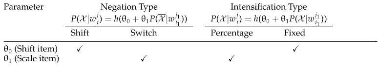
Table 2 illustrates how the regression based polarity model represents different negation and intensification methods. For a specific rule, the parameters and the com-positional method are automatically learned from data (Section 4.2.3) instead of setting them manually as in previous work (Taboada et al. 2011). In a similar way, this method can handle the contrast. For example, the inference rule forN→P but Nis:

(N→PbutN) [i1,P,j1]Φ1 [i2,N,j2]Φ2

[i,N,j] (

P(N|wj_i)=h(θ₀+θ₁P(P|wj1_i1)+θ₂P(N|wj2_i2))

P(P|wj_i)=1−P(N|wj_i)

(17)

where the polarity probability of the ruleN→P but Nis computed byP(N|wj_i)=h(θ₀+

θ₁P(P|wj1_i1)+θ₂P(N|wj2_i2)). It can express the contrast relation by specific parametersθ₀, θ₁, andθ₂.

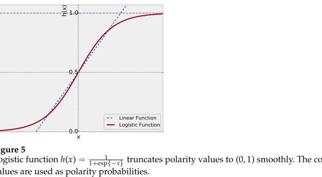
[image:15.486.50.437.594.664.2]

It should be noted that a linear regression model could turn out to be problem-atic, as it may produce unreasonable results. For example, if we do not add any constraint, we may getP(N|wj_i)=−0.6+P(P|wj_i+1). WhenP(P|wj_i+1)=0.55, we will getP(N|wj_i)=−0.6+0.55=−0.05. This conflicts with the definition that the polarity probability ranges from zero to one. Figure 5 intuitively shows that the logistic function truncates polarity values to (0, 1) smoothly.

Table 2

The check mark means the parameter of the polarity model can capture the corresponding intensification type and negation type. Shift itemθ₀can handle shift negation and fixed intensification, and scale itemθ₁can model switch negation and percentage intensification.

Parameter Negation Type

P(X|wj_i)=h(θ0+θ1P(X|w

j₁ i1))

Intensification Type P(X|wj_i)=h(θ0+θ1P(X|w

j₁ i1))

Shift Switch Percentage Fixed

θ0(Shift item) X X

x 0.0 0.5 1.0

h(x)

[image:16.486.57.384.61.241.2]

Linear Function Logistic Function

Figure 5

Logistic functionh(x)= 1

1+exp{−x}truncates polarity values to (0, 1) smoothly. The computed

values are used as polarity probabilities.

3.5 Constraints

We incorporate additional constraints into the parsing model. Those are used as pruning conditions in the derivation process not only to improve efficiency but also to force the derivation towards the correct direction. We expand the inference rules in Section 3.4 as,

(r) H1Φ1 . . . HKΦK

[i,X,j]Φ C (18)

where C is aside condition. The constraints are interpreted in a Boolean manner. If the constraintCis satisfied, the rule can be used, otherwise, it cannot. We define two constraints in the parsing model.

First, in the parsing process, the polarity label of text span wj_i obtained by the polarity model (Section 3.4) should be consistent with the non-terminal X (N or P) on the left hand side of the rule. To distinguish between the polarity labels and the non-terminals, we denote the corresponding polarity label of non-terminal X as X. Following this notation, we describe the first constraint as

C1:P(X|wji)>P(X|w j

i) (19)

whereX is the opposite polarity ofX. For instance, if ruleP→not Nmatches the text spanwj_i, the polarity calculated by the polarity model should be consistent withP, i.e., the polarity obtained by the polarity model should be positive (P).

Second, when we apply the combination rules, the polarity strength of subspans needs to exceed a predefined thresholdτ(≥0.5). Specifically, for combination rulesX→

wi1_i X1wi2_j1X2w_j2j andX→wi1_i X1wj_j1, we define the second constraint as

C2 :P(Xk|wikjk)> τ,k=1,. . .,K (20)

τ, we regard the polarity of phrasewjk_ik as neutral. For instance, we do not want to use the combination ruleP→a lot ofPorN→a lot ofNfor the phrasea lot of people. This constraint avoids improperly using the combination rules for neutral phrases. Notably, whenτis set as 0.5, this constraint is the same as the first one in Equation (19).

As shown in Figure 6, we add these two constraints to the inference rules. The OOV rules do not have any constraints, and the constraintC1is applied for all the other rules. The constraintC2is only applied for the combination rules.

3.6 Decoding Algorithm

In this section, we summarize the decoding algorithm in Algorithm 1. For a sentences, the CYK algorithm and dynamic programming are used to obtain the sentiment tree with the highest score. To be specific, the modified CYK parsing model parses the input sentence to sentiment trees in a bottom–up manner—that is, from short to long text spans. For every text spanwj_i, we match the rules in the sentiment grammar (Section 3.1) to generate the candidate set. Their polarity values are calculated using the polarity model described in Section 3.4. We also use the constraints described in Section 3.5 to prune search paths. The constraints improve the efficiency of the parsing algorithm and make derivations that meet our intuition.

(X→wj_i)

[i,X,j]P(X|w_ij)=P˜(X|wj_i)C1

(X→wi1_iX1wjj1) [i1,X1,j1]Φ1 [i,X,j]P(X|wj_i)=h(θ₀+θ₁P(X₁|wj1_i1))C1

∧C2

(X→wi1_i X1wi2j1X2w

j

j2) [i1,X1,j1]Φ1 [i2,X2,j2]Φ2 [i,X,j]P(X|wj_i)=h(θ₀+θ₁P(X₁|wj1_i1)+θ₂P(X₂|wj2_i2))C1

∧C2

(X→X1X2) [i,X1,k]Φ1 [k,X2,j]Φ2

[i,X,j]P(X|wj_i)= P(X|wki)P(X|w j k) P(X|wk

i)P(X|w j

k)+P(X|wki)P(X|w j k)

C1

(E→wj_i) [i,E,j]◦ ◦

(X→EX1) [i,E,k]◦ [k,X1,j]Φ1 [i,X,j]P(X|w_ij)=P(X|wj_k) C1 (X→X1E) [i,X1,k]Φ1 [k,E,j]◦

[i,X,j]P(X|wj_i)=P(X|wk i)

C1

whereh(x)= 1

1+exp{−x}is a logistic function,◦represents the absence, andX,X1,X2

[image:17.486.62.386.323.618.2]

representNorP.As specified in the polarity model, we haveP(X|wj_i)=1−P(X|wj_i).

Figure 6

Algorithm 1Decoding Algorithm Input: wn₀: Sentence

Output: Polarity of the input sentence 1: score[, , ]← {}

2: forl←1. . .ndo .Modified CYK algorithm

3: for alli,j s.t. j−i=ldo

4: for allinferable rule (r)_[H1_i,X..._,j]HK forwj_ido

5: Φ←calculate polarity value forr .Polarity model

6: ifconstraints are satisfiedthen .Constraint

7: sc←compute score for this derivation by ranking model .Ranking model

8: ifsc>score[i,j,X]then 9: score[i,j,X]←sc

10: returnarg max_X∈{N,P}score[0,X,n]

The features in the ranking model (Section 4.1.1) decompose along the structure of the sentiment tree. So the dynamic programming technique can be used to compute the derivation tree with the highest ranking score. For a span, the scores of its subspans are used to calculate the local scores of its derivations. For example, the score of the derivation (r) [i1,P_[,_ij1_,X] [_,j]i2,N,j2] isscore[i1,j1,P]+score[i2,j2,N]+scorer, wherescore[i,j,X] is the highest score of text span wj_i that is derived to the non-terminalX, and scorer is the score of applying the ruler. As described in Section 3.3, the score of using ruleris

scorer=φ(wj_i,r)Tψ, whereφ(wj_i,r) is the feature vector of using the rulerfor the span

wj_i, andψis the weight vector of the ranking model. Thekhighest score trees satisfying the constraints are stored inscore[, , ] for decoding the longer text spans. After finishing the CYK parsing, arg max_X∈{N,P}score[0,n,X] is regarded as the polarity label of input sentence. The time complexity is the same as the standard CYK’s.

4. Model Learning

We described the statistical sentiment parsing framework in Section 3. We present the model learning process in this section. The learning process consists of two steps. First, the sentiment grammar and the polarity model are learned from data. In other words, the rules and the parameters used to compute polarity values are learned. These basic sentiment building blocks are then used to build the parse trees. Second, we estimate the parameters of the ranking model using the sentence and polarity label pairs. At this stage, we concentrate on learning how to score the parse trees based on the learned sentiment grammar and polarity model.

Section 4.1 shows the features and the parameter estimation algorithm used in the ranking model. Section 4.2 illustrates how to learn the sentiment grammar and the polarity model.

4.1 Ranking Model Training

candidates. Then, we describe the objective function used in the optimization algorithm. Finally, we introduce the algorithm for parameter estimation using the gradient-based method.

4.1.1 Features.We extract a feature vectorφ(s,t)∈Rd_{for each parse treetof sentences.}

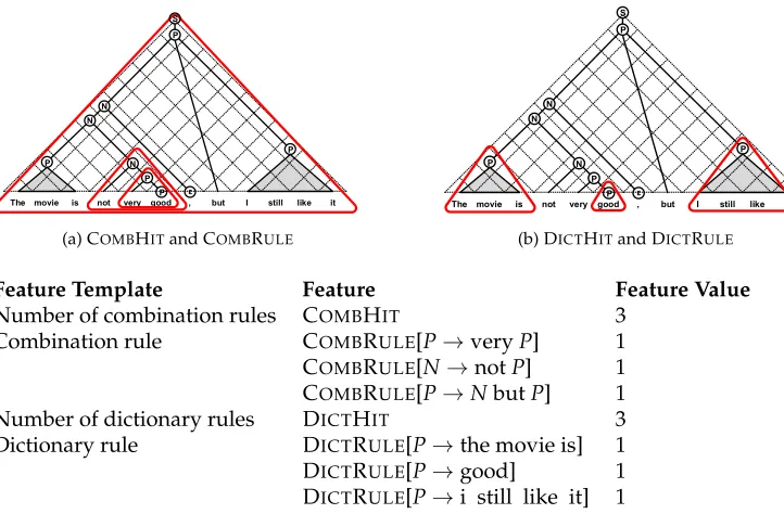
The feature vector is used in the log-linear model. In Figure 7, we present the features extracted for the sentenceThe movie is not very good, but i still like it. The features are organized into feature templates. Each of them contains a set of features. These feature templates are shown as follows:

r

_{COMBHIT: This feature is the total number of combination rules used int.}

r

_{COMBRULE: It contains features}{COMBRULE[r] :ris a combination rule},

each of which fires on the combination rulerappearing int.

r

_{DICTHIT: This feature is the total number of dictionary rules used int.}

r

_{DICTRULE: It contains features}{DICTRULE[r] :ris a dictionary rule}, each

of which fires on the dictionary rulerappearing int.

These features are generic local patterns that capture the properties of the senti-ment tree. Another intuitive lexical feature template is [combination rule + word]. For instance, P→very P(good) is a feature that lexicalizes the non-terminal P to good. However, if this feature is fired frequently, the phrasevery goodwould be learned as a dictionary rule and can be used in the decoding process. So we do not use this feature template in order to reduce the feature size. It should be noted that these features

The movie is not very good , but I still like it P

P P ε

P P

N N

N S

(a) COMBHITand COMBRULE

The movie is not very good , but I still like it P

P P ε

P P

N N

N S

(b) DICTHITand DICTRULE

Feature Template Feature Feature Value

Number of combination rules COMBHIT 3

Combination rule COMBRULE[P→veryP] 1 COMBRULE[N→notP] 1 COMBRULE[P→NbutP] 1

Number of dictionary rules DICTHIT 3

[image:19.486.57.418.389.626.2]

Dictionary rule DICTRULE[P→the movie is] 1 DICTRULE[P→good] 1 DICTRULE[P→i still like it] 1

Figure 7

decompose along structures of sentiment trees, enabling us to use dynamic program-ming in the CYK algorithm.

4.1.2 Objective Function.We design the ranking model upon the log-linear model to score candidate sentiment trees. In the training dataD, we only have the input sentencesand its polarity labelL_s. The forms of sentiment parse trees, which can obtain the correct sentiment polarity, are unobserved. So we work with the marginal log-likelihood of obtaining the correct polarity labelL_s,

logp(L_s|s;T,ψ)=logp(t∈TLs_(s)|s;T,ψ)

=A(ψ;s,TLs_{)−A(ψ;s,T)} (21)

where TLs _{is the set of candidate trees whose prediction labels are L}

s, andA(ψ;s,T)

(Equation (10)) is the log-partition function with respect toT(s).

Based on the marginal log-likelihood function, the objective functionO(ψ,T) con-sists of two terms. The first term is the sum of marginal log-likelihood over training instances that can obtain the correct polarity labels. The second term is a L2-norm regularization term on the parametersψ. Formally,

O(ψ,T)= X

(s,Ls)∈D TLs_(s)6=∅

logp(L_s|s;T,ψ)−λ

2kψk 2 2

(22)

To learn the parametersψ, we use a gradient-based optimization method to max-imize the objective functionO(ψ,T). According to Wainwright and Jordan (2008), the derivative of the log-partition function is the expected feature vector

∂O(ψ,T)

∂ψ =

X

(s,Ls)∈D TLs_(s)6=∅

(Ep(t|s;TLs_,ψ)[φ(s,t)]−E_p(t|s;T,ψ)[φ(s,t)])−λψ (23)

whereEp(x)[f(x)]=Pxp(x)f(x) for discretex.

4.1.3 Parameter Estimation.The objective functionO(ψ,T) is not concave (nor convex), hence the optimization potentially results in a local optimum. Stochastic Gradient De-scent (SGD; Robbins and Monro 1951) is a widely used optimization method. The SGD algorithm picks up a training instance randomly, and updates the parameter vectorψ according to

ψ_j(t+1)=ψ_j(t)+α

∂O(ψ) ∂ψ_j |ψ=ψ(t)

(24)

where αis the learning rate, and ∂_∂ψO(ψ)

j is the gradient of the objective function with

steps when we meet a feature many times. In order to compute efficiently, a diagonal approximation version of AdaGrad is used. The update rule is

ψ_j(t+1)=ψ_j(t)+α_q 1 G_j(t+1)

∂O(ψ)

∂ψ_j |ψ=ψ(t)

G_j(t+1)=G(_jt)+

∂O(ψ)

∂ψ_j |ψ=ψ(t)

2

(25)

where we introduce an adaptive termG(_jt).G(_jt)becomes larger along with updating, and decreases the update step for dimensionj. Compared with SGD, the only cost is to store and updateG(_jt)for each parameter.

To train the model, we use the method proposed by Liang, Jordan, and Klein (2013). With the candidate parse trees and objective function, the parametersψare updated to make the parsing model favor correct trees and give them a higher score. Because there are many parse trees for a sentence, we need to calculate Equation (23) efficiently. As indicated in Section 4.1.1, the features decompose along the structure of sentiment trees. So dynamic programming can be utilized to computeEp(t|s;T,ψ)[φ(s,t)] of Equation (23). However, the first expectation termEp(t|s;TLs_,ψ)[φ(s,t)] sums over the candidates that obtain the correct polarity labels. As this constraint does not decompose along the tree structure, there is no efficient dynamic program for this. Instead of searching all the parse trees spanning s, we use beam search to approximate this expectation. Beam search is a best-first search algorithm that explores at most K paths (K is the beam size). It keeps the local optimums to reduce the huge search space. Specifically, the beam search algorithm generates theK-best trees with the highest scoreφ(s,t)T_ψfor

each span. These local optimums are used recursively in the CYK process. TheK-best trees for the whole span are regarded as the candidate set ˜T. Then ˜Tand ˜TLs_{are used to}

approximate Equation (23) as in Liang, Jordan, and Klein (2013).

The intuition behind this parameter estimation algorithm lies in: (1) if we have better parameters, we can obtain better candidate trees; (2) with better candidate trees, we can learn better parameters. Thus the optimization problem is solved in an iterative manner. We initialize the parameters as zeros. This leads to a random search and gen-erates random candidate trees. With the initial candidates, the two steps in Algorithm 2 lead the parametersψtowards the direction achieving better performance.

4.2 Sentiment Grammar Learning

Algorithm 2Ranking Model Learning Algorithm

Input: D: Training data{(s,L_s)},S: Maximum number of iteration Output: ψ: Parameters of the ranking model

1: ψ(0)_{←(0, 0,. . ., 0)}T

2: repeat

3: (s,L_s)←randomly select a training instance inD

4: T˜(t)←BEAMSEACH(s,ψ(t)) .Beam search to generate K-best candidates 5: G(_jt+1)←G_j(t)+∂O_∂ψ(ψ, ˜T(t))

j |ψ=ψ(t)

2

6: ψ(_jt+1)←ψ_j(t)+α 1

q G(tj+1)

∂O(ψ, ˜T(t)₎

∂ψj |ψ=ψ(t)

.Update parameters using

AdaGrad 7: t←t+1 8: untilt>S

9: returnψ(T)

sentences annotated with sentiment polarity labels are relatively easy to obtain, and we use them as our input to learn dictionary rules and combination rules.

We first present the basic idea behind the algorithm we propose. People are likely to express positive or negative opinions using very simple and straightforward sentiment expressions again and again in their reviews. Intuitively, we can mine dictionary rules from these massive review sentences by leveraging the redundancy characteristics. Furthermore, there are many complicated reviews that contain complex sentiment structures (e.g., negation, intensification, and contrast). If we already have dictionary rules on hand, we can use them to obtain basic sentiment information for the fragments within complicated reviews. We can then extract combination rules with the help of the dictionary rules and the sentiment polarity labels of complicated reviews. Because the simple and straightforward sentiment expressions are often coupled with complicated expressions, we need to conduct dictionary rule mining and the combination rule mining in an iterative way.

4.2.1 Dictionary Rule Learning. The dictionary rules GD are basic sentiment building blocks used in the parsing process. Each dictionary rule in GD is in the form X→f, wheref is a sentiment fragment. We use the polarity probabilitiesP(N|f) andP(P|f) in the polarity model. To buildGD, we regard all the frequent fragments whose occurrence frequencies are larger thanτ_f and lengths range from 1 to 7 as the sentiment fragments. We further filter the phrases formed by stop words and punctuations, which are not used to express sentiment.

For a balanced data set, the sentiment distribution of a candidate sentiment frag-mentf is calculated by

P(X|f)= #(f,X)+1

#(f,N)+#(f,P)+2 (26)

where X∈ {N,P}, and #(f,X) denotes the number of reviews containing f with X

We do not learn the polarity probabilitiesP(N|f) andP(P|f) by directly counting occurrence frequency. For example, in the review sentencethis movie is not good (nega-tive), the naive counting method increases the count #(good,N) in terms of the polarity of the whole sentence. Moreover, because of the common collocation not as good as

(negative) in movie reviews, as good as is also regarded as negative if we count the frequency directly. The examples indicate why some polarity probabilities of phrases counting from data are different from our intuitions. These unreasonable polarity probabilities also make trouble for learning the polarity model. Consequently, in order to estimate more reasonable probabilities, we need to take the compositionality into consideration when learning sentiment fragments.

Following this motivation, we ignore the count #(f,X), if the sentiment fragment

f iscovered by a negation rule rthat negates the polarity off. The word coverhere means thatf is derived within a non-terminal of the negation ruler. For instance, the negation ruleN→notPcovers the sentiment fragmentgoodin the sentencethis is not a good movie(negative), that is, thegoodis derived fromPof this negation rule. So we ignore the occurrence for #(good,N) in this sentence. It should be noted that we still increase the count for #(not good,N), because there is no negation rule covering the fragmentnot good.

As shown in Algorithm 3, we learn the dictionary rules and their polarity probabil-ities by counting the frequencies in negative and positive classes. Only the fragments whose occurrence numbers are larger than thresholdτ_f are kept. Moreover, we take the combination rules into consideration to acquire more reasonable GD. Notably, a subsequence of a frequent fragment must also be frequent. This is similar to the key insight in the Apriori algorithm (Agrawal and Srikant 1994). When we learn the dic-tionary rules, we can count the sentiment fragments from short to long, and prune the infrequent fragments in the early stages if any subsequence is not frequent. This pruning method accelerates the dictionary rule learning process and makes the procedure fit in memory.

Algorithm 3Dictionary Rule Learning

Input: D: Data set,GC: Combination rules,τf: Frequency threshold

Output: GD: Dictionary rules

1: functionMINEDICTIONARYRULES(D,GC) 2: GD0← {}

3: for(s,L_s) inDdo .s:w0w1· · ·w|s|−1,Ls: Polarity label ofs

4: for alli,j s.t. 0≤i<j≤ |s|do .wj_i:wiwi+1· · ·wj−1 5: ifno negation rule inG_Ccoverswj_ithen

6: #(wj_i,Ls)++

7: addwj_itoGD0 8: GD← {}

9: forf inGD0do 10: if#(f,·)≥τ_f then

11: computeP(N|f) andP(P|f) using Equation (26)

12: add dictionary rule (Lf →f) toGD .Lf =arg maxX∈{N,P}P(X|f)

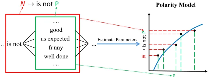
4.2.2 Combination Rule Learning. The combination rulesGC are generalizations for the dictionary rules. They are used to handle the compositionality and process unseen phrases. The learning of combination rules is based on the learned dictionary rules and their polarity values. The sentiment fragments are generalized to combination rules by replacing the subsequences of dictionary rules with their polarity labels. For instance, as shown in Figure 8, the fragmentsis not (good/as expected/funny/well done)are all negative. After replacing the subspansgood,as expected,funny, andwell donewith their polarity labelP, we can learn the negation ruleN→is notP.

We present the combination rule learning approach in Algorithm 4. Specifically, the first step is to generate combination rule candidates. For every subsequence wj_i

of sentiment fragment f, we replace it with the corresponding non-terminal L_wj i if P(L

wji

|wj_i) is larger than the thresholdτ_p, and we can getwi₀L_wj iw

|f|

j . Next, we compare

the polarityL wji with

L_f. IfL_f 6=L

wji, we regard the ruleLf

→wi₀L_wj iw

|f|

j as a negation

rule. Otherwise, we further compare their polarity values. If this rule makes the polarity value become larger (or smaller), it will be treated as a strengthen (or weaken) rule. To obtain the contrast rules, we replace two subsequences with their polarity labels in a similar way. If the polarities of these two subsequences are different, we categorize this rule to the contrast type. Notably, these two non-terminals cannot be next to each other. After these steps, we get the rule candidate setGC0and the occurrence number of each rule. We then filter the rule candidates whose occurrence frequencies are too small, and assign the rule types (negation, strengthen, weaken, and contrast) according to their occurrence numbers.

4.2.3 Polarity Model Learning. As shown in Section 3.4, we define the polarity model to calculate the polarity probabilities using the sentiment grammar. In this section, we present how to learn the parameters of the polarity model for the combination rules.

P

𝑁

→

is

no

t

P

𝑁

→

is not

P

… is not

…

…

…

good

as expected

funny

well done

Estimate Parameters

[image:24.486.51.412.414.549.2]

Polarity Model

Figure 8

We replace the subsequences with their polarity labels for frequent sentiment fragments. As shown here, we replacegood,as expected,funny, andwell donewith their polarity labelP. Then we compare the polarity probabilities of subfragments with the whole fragments, such asgoodandis not good, to determine whether it is a negation rule, strengthen rule, or weaken rule. After obtaining the rule, we use polarity probabilities of these compositional examples as training data to estimate parameters of the polarity model. In this, P(P|good),P(N|is not good)

, P(P|as expected),P(N|is not as expected)

, P(P|funny),P(N|is not funny)

Algorithm 4Combination Rule Learning

Input: D: Data set,G_D: Dictionary rules,τ_p,τ_∆,τ_r,τ_c: Thresholds Output: GC: Combination rules

1: functionMINECOMBINATIONRULES(D,GD) 2: GC0← {}

3: for(X→f) inGDdo .f :w0w1· · ·w|f|−1

4: for alli,j s.t. 0≤i<j≤ |f|do 5: ifP(L_wj

i

|wj_i)> τ_pthen .Polarity labelL_wj i

=arg maxX∈{N,P}P(X|w j i)

6: r:X→wi

0Lwj_iw |f|

j .Non-terminalLwj_i =arg maxX∈{N,P}P(X|w j i)

7: ifX 6=L

wj_ithen

8: #(r,negation)++

9: else ifP(X|f)>P(L wj_i|w

j

i)+τ∆then

10: #(r,strengthen)++

11: else ifP(X|f)<P(L wji

|wj_i)−τ_∆then

12: #(r,weaken)++

13: addrtoGC0

14: for alli0,j0,i1,j1 s.t. 0≤i0<j0<i1 <j1 ≤ |f|do 15: ifP(L

wj0 i₀

|wj0_i0)> τ_pandP(L wj1

i₁

|wj1_i1)> τ_pthen

16: r:X→wi0₀L_wj₀ i₀

wi1_j0L_wj₁ i₁

w|_j1f| .Replacewj0_i0,wj1_i1with the non-terminals

17: ifL

wj0 i₀

6

=L

wj1 i₁

then

18: #(r,contrast)++

19: addrtoGC0 20: GC← {}

21: forrinGC0do

22: if#(r,·)> τ_randmax

T

#(r,T)

#(r) > τcthen 23: addrtoG_C

24: returnGC

As shown in Figure 8, we learn combination rules by replacing the subsequences of frequent sentiment fragments with their polarity labels. Both the replaced fragment and the whole fragment can be found in the dictionary rules, so their polarity probabilities have been estimated from data. We can use them as our training examples to figure out how context changes the polarity of replaced fragment, and learn parameters of the polarity model.

We describe the polarity model in Section 3.4. To further simplify the notation, we denote the input vectorx=(1,P(X₁|wj1_i1),. . .,P(X_K|wjK_iK))T_{, and the response value asy.}

Then we can rewrite Equation (15) as

hθ(x)= 1

where hθ(x) is the polarity probability calculated by the polarity model, and θ= (θ₀,θ₁,. . .,θ_K)T _{is the parameter vector. Our goal is to estimate the parameter vector}

θof the polarity model.

We fit the model to minimize the sum of squared residuals between the predicted polarity probabilities and the values computed from data. We define the cost function as

J(θ)=1

2 X

m

(hθ(xm)−ym)2 ₍₂₈₎

where xm,ym

is them-th training instance.

The gradient descent algorithm is used to minimize the cost function J(θ). The partial derivative ofJ(θ) with respect toθ_jis

∂J(θ) ∂θ_j =

X

m

hθ(xm)−ym

∂hθ(xm)

∂θ_j

=X

m

hθ(xm)−ym

hθ(xm) 1−hθ(xi)

∂θTxm ∂θ_j

=X

m

hθ(xm)−ym

hθ(xm) (1−hθ(xm))xmj

(29)

We set the initial θ as zeros, and start with it. We use the Stochastic Gradient Descend algorithm to minimize the cost function. For the instance (x,y), the parameters are updated using

θ_j(t+1)=θ_j(t)−α

∂J(θ) ∂θ_j |θ=θ(t)

=θ_j(t)−α(h_θ(t)(x)−y)h_θ(t)(x) 1−h_θ(t)(x)

xj

(30)

whereαis the learning rate, and it is set to 0.01 in our experiments. We summarize the learning method in Algorithm 5. For each combination rule, we iteratively scan

Algorithm 5Polarity Model Learning Algorithm

Input: G_C: Combination rules,ε: Stopping condition,α: Learning rate Output: θ: Parameters of the polarity model

1: functionESTIMATEPOLARITYMODEL(G_C) 2: for allcombination ruler∈GCdo 3: θ(0)←(0, 0,..., 0)T

4: repeat

5: x,y

←randomly select a training instance

6: θ_j(t+1)←θ_j(t)−α(hθ(t)(x)−y)h_θ(t)(x) 1−h_θ(t)(x)

xj

7: t←t+1

8: untilθ(t+1)−θ(t) 2 2< ε

Algorithm 6Sentiment Grammar Learning

Input: D: Data set{(s,L_s)},T: Maximum number of iteration .L_s: Polarity label ofs

Output: GD: Dictionary rules,GC: Combination rules 1: GC← {}

2: repeat

3: GD←MINEDICTIONARYRULES(D,GC) .Algorithm 3 4: GC←MINECOMBINATIONRULES(D,GD) .Algorithm 4 5: untiliteration number exceedsT

6: ESTIMATEPOLARITYMODEL(GC) .Algorithm 5

7: returnGD,GC

through the training examples x,y

in a random order, and update the parameters θ according to Equation (30). The stopping condition is θ(t+1)−θ(t)

2

2 < ε, which indicates the parameters become stable.

4.2.4 Summary of the Grammar Learning Algorithm.We summarize the grammar learning process in Algorithm 6, which learns the sentiment grammar in an iterative manner.

We first learn the dictionary rules and their polarity probabilities by counting the frequencies in negative and positive classes. Only the fragments whose occurrence num-bers are larger than the thresholdτ_f are kept. As mentioned in Section 4.2.1, the context can essentially change the distribution of sentiment fragments. We take the combination rules into consideration to acquire more reasonableGD. In the first iteration, the set of combination rules is empty. Therefore, we have no information about compositionality to improve dictionary rule learning. The initialGDcontains some inaccurate sentiment distributions. Next, we replace the subsequences of dictionary rules to their polarity labels, and generalize these sentiment fragments to the combination rulesGC as illus-trated in Section 4.2.2. At the same time, we can obtain their compositional types and learn parameters of the polarity model. We iterate over these two steps to obtain refined

G_DandG_C.

5. Experimental Studies

In this section, we describe experimental results on existing benchmark data sets with extensive comparisons with state-of-the-art sentiment classification methods. We also present the effects of different experimental settings in the proposed statistical senti-ment parsing framework.

5.1 Experiment Set-up

We describe the data sets in Section 5.1.1, the experimental settings in Section 5.1.2, and the methods used for comparison in Section 5.1.3.

reviews from Rotten Tomatoes3 _{and IMDb.}4 _{We balance the positive and negative} instances in the training data set to mitigate the problem of data imbalance. Moreover, the Stanford Sentiment Treebank5contains polarity labels of all syntactically plausible phrases. In addition, we use the MPQA6data set for the phrase-level task. We describe these data sets as follows.

RT-C: 436,000 critic reviews from Rotten Tomatoes. It consists of 218,000 negative and 218,000 positive critic reviews. The average review length is 23.2 words. Critic reviews from Rotten Tomatoes contain a label (Rotten: Negative, Fresh: Positive) to indicate the polarity, which we use directly as the polarity label of corresponding reviews.

PL05-C: The sentence polarity data set v1.0 (Pang and Lee 2005) contains 5,331 positive and 5,331 negative snippets written by critics from Rotten Tomatoes. This data set is widely used as the benchmark data set in the sentence-level polarity classification task. The data source is the same as RT-C.

SST: The Stanford Sentiment Treebank (Socher et al. 2013) is built upon PL05-C. The sentences are parsed to parse trees. Then, 215,154 syntactically plausible phrases are extracted and annotated by workers from Amazon Mechanical Turk. The experimental settings of positive/negative classification for sentences are the same as in Socher et al. (2013).

RT-U: 737,806 user reviews from Rotten Tomatoes. Because we focus on sentence-level sentiment classification, we filter out user reviews that are longer than 200 char-acters. The average length of these short user reviews from Rotten Tomatoes is 15.4 words. Following previous work on polarity classification, we use the review score to select highly polarized reviews. For the user reviews from Rotten Tomatoes, a negative review has a score<2.5 out of 5, and a positive review has a score>3.5 out of 5.

IMDB-U: 600,000 user reviews from IMDb. The user reviews in IMDb contain comments and short summaries (usually a sentence) to summarize the overall sentiment expressed in the reviews. We use the review summaries as the sentence-level reviews. The average length is 6.6 words. For user reviews of IMDb, a negative review has a score <4 out of 10, and a positive review has a score>7 out of 10.

C-TEST: 2,000 labeled critic reviews sampled from RT-C. We use C-TEST as the testing data set for RT-C. Note that we exclude these from the training data set (i.e., RT-C).

U-TEST: 2,000 manually labeled user reviews sampled from RT-U. User reviews often contain some noisy ratings compared with critic reviews. To eliminate the ef-fect of noise, we sample 2,000 user reviews from RT-U, and annotate their polarity labels manually. We use U-TEST as a testing data set for RT-U and IMDB-U, which are both user reviews. Note that we exclude them from the training data set (i.e., RT-U).

MPQA: The opinion polarity subtask of the MPQA data set (Wiebe, Wilson, and Cardie 2005). The authors manually annotate sentiment polarity labels for the ex-pressions (i.e., sub-sentences) within a sentence. We regard the exex-pressions as short sentences in our experiments. There are 7,308 negative examples and 3,316 positive examples in this data set. The average number of words per example is 3.1.

3http://www.rottentomatoes.com.

4http://www.imdb.com.

5http://nlp.stanford.edu/sentiment/treebank.html.

[image:29.486.53.437.120.209.2]

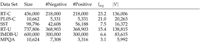
Table 3

Statistical information of data sets. #Negative and #Positive are the number of negative instances and positive instances, respectively.lavgis average length of sentences in the data set, and|V|is

the vocabulary size.

Data Set Size #Negative #Positive lavg |V|

RT-C 436,000 218,000 218,000 23.2 136,006

PL05-C 10,662 5,331 5,331 21.0 20,263

SST 98,796 42,608 56,188 7.5 16,372

RT-U 737,806 368,903 368,903 15.4 138,815

IMDB-U 600,000 300,000 300,000 6.6 83,615

MPQA 10,624 7,308 3,316 3.1 5,992

Table 3 shows the summary of these data sets, and all of them are publicly available athttp://goo.gl/WxTdPf.

5.1.2 Settings. To compare with other published results for PL05-C and MPQA, the training and testing regime (10-fold cross-validation) is the same as in Pang and Lee (2005), Nakagawa, Inui, and Kurohashi (2010) and Socher et al. (2011). For SST, the regime is the same as in Socher et al. (2013). We use C-TEST as the testing data for RT-C, and U-TEST as the testing data for RT-U and IMDB-U. There are a number of settings that have trade-offs in performance, computation, and the generalization power of our model. The best settings are chosen by a portion of training split data that serves as the validation set. We provide the performance comparisons using different experimental settings in Section 5.4.

Number of training examples: The size of training data has been widely recognized as one of the most important factors in machine learning-based methods. Generally, using more data leads to better performance. By default, all the training data is used in our experiments. We use the same size of training data in different methods for fair comparisons.

Number of training iterations (T): We use AdaGrad (Duchi, Hazan, and Singer 2011) as the optimization algorithm in the learning process. The algorithm starts with randomly initialized parameters, and alternates between searching candidate sentiment trees and updating parameters of the ranking model. We treat one-pass scan of training data as an iteration.

Beam size (K): The beam size is used to make a trade-off between the search space and the computation cost. Moreover, an appropriate beam size can prune unfavorable candidates. We setK=30 in our experiments.

Regularization (λ): The regularization parameterλin Equation (22) is used to avoid over-fitting. The value used in the experiments is 0.01.