Direct Fuzzy Adaptive Control for Standalone
Wind Energy Conversion Systems
Hoa M. Nguyen,
Member, IAENG
and D. S. Naidu.
Abstract—This paper presents a direct fuzzy adaptive control for standalone Wind Energy Conversion Systems (WECS) with Permanent Magnet Synchronous Generators (PMSG). The problem of maximizing power conversion from intermittent wind of time-varying, highly nonlinear WECS is dealt with by an adaptive control algorithm. The adaptation is designed based on the Lyapunov theory and carried out by the fuzzy logic technique. Comparison between the proposed method and the feedback linearization method is shown by numerical simulations verifying the effectiveness of the suggested adaptive control scheme.
Index Terms—wind energy conversion system, permanent magnet synchronous generators, fuzzy logic, nonlinear adaptive control.
I. INTRODUCTION
W
IND energy is a renewable energy source. It has developed significantly in the last few decades and now has the fastest growth among other renewable energy sources [1].Wind energy is harvested by WECS or wind turbines. These wind energy converters can be classified as grid-connected or standalone depending on their connections to utility grids or local grids. Nowadays most WECS are connected to utility grids. However there is still demand for standalone WECS which provide electrical power for remote areas where utility grids cannot reach. To guarantee continuous energy supply, standalone WECS are combined with other energy sources such as battery storage systems, solar energy systems, diesel generators, etc. resulting in Hy-brid Wind Energy Systems (HWES). Due to the presence of other energy sources, the control of HWES is quite different from that of grid-connected WECS. Beside attempting to capture as much power as possible, controllers need to ensure constant power flow to local loads. A number of control strategies has been proposed for HWES in [2], [3], [4]. Most of these works focus on the interaction between WECS and storage systems. Meanwhile, authors in [5] deal with the control of maximizing the power conversion of WECS in HWES based on the nonlinear feedback linearization control method.
The adaptive control is an attractive control which provides controllers ability to learn as systems and/or environments change [6]. This feature is particularly useful for WECS which are immersed in highly stochastic wind surroundings. Different adaptive structures were presented to WECS in [7]–[12]. Basically these works study adaptive Proportional Integral Derivative (PID) control using fuzzy logic [7], [8]
Manuscript received July 02, 2012; revised July 31, 2012.
Hoa M. Nguyen is with the Department of Electrical Engineering, Idaho State University, Pocatello, ID, 83201 USA e-mail: [email protected].
D. S. Naidu is with the Department of Electrical Engineering, School of Engineering, Idaho State University, Pocatello, ID, 83201 USA e-mail: [email protected].
or neural networks [9]–[12] to tune PID parameters. Our paper focuses on an adaptive control scheme based on the input-output linearization control where the adaptive rule is designed based on theLyapunovanalysis. The chosen HWES is the same as in [5]. The results of the adaptive control will be compared to that of the feedback linearization control in [5] proving advantages of the proposed control.
The paper is organized as follows. Section II describes the HWES and the standalone PMSG-based WECS nonlinear model. The adaptive control design is presented in Section III followed by its application to the standalone WECS in Section IV. Based on simulation results shown in Section V, some discussions and conclusions are drawn in Section VI.
II. STANDALONEWINDENERGYCONVERSIONSYSTEM MODELING
A HWES includes a WECS interacting with another source of energy as shown in Fig. 1. Due to the output power from the WECS fluctuating according to wind changes, other energy sources such as battery or solar systems or diesel generators must be added to ensure a constant power supply to the local grid. Maximum power conversion of the WECS is obtained by adjusting the generator speedωgas wind speed
V changes. This is achieved by modifying the equivalent load at the generator terminal via power electronics converters. The equivalent standalone WECS is depicted in Fig. 2 where
RLandLLare the equivalent load resistance and inductance, respectively. The equivalent load resistance is considered the control input for the control system.
The dynamic model of the standalone WECS is obtained by combining the aerodynamics, drive train dynamics and generator dynamics. Note that the power electronics dy-namics is ignored because it is much faster than the other dynamics.
The aerodynamics converts wind flows into aerodynamic torque and mechanical power given respectively as
Tr =
1
2ρπR
3V2C
Q(λ, β), (1)
Pr =
1
2ρπR
2V3C
P(λ, β), (2)
where Tr is the aerodynamic torque, ρ is the air density,
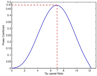
R is the radius of the wind rotor swept area, V is the wind speed, CQ(λ, β) is the torque coefficient, Pr is the mechanical power, andCP(λ, β)is the power coefficient. It is seen that both torque and power coefficient are functions of the so-called tip-speed ratioλand pitch angle of the wind rotor blades β. The tip-speed ratio is defined as the ratio between the speed at the tip of blades and the wind speed, which is given as
λ=ωrR
Fig. 1. Hybrid Wind Energy System
Fig. 2. Standalone WECS
where ωr is the wind rotor rotational speed. However for the optimal power conversion purpose the torque coefficient in (1) is only dependent on the tip-speed ratio and can be approximated as the following sixth-order polynomial function of the tip-speed ratio [5]
CQ(λ) = a6λ6+a5λ5+a4λ4+a3λ3+a2λ2
+a1λ+a0. (4)
The power coefficient CP(λ) has its maximum value at the so-called optimal tip-speed ratioλ∗as illustrated in Fig. 3. Therefore, to maximize the power conversion, the WECS must operate at the optimal tip-speed ratio. However, when the wind speed changes, the tip-speed ratio is perturbed away from the optimal value as seen from (3). To maintain the optimal tip-speed ratio, the wind rotor speed ωr must be adjusted by the control system.
The standalone PMSG model in thedirectandquadrature
(d,q) frame is given as [5]
d
dtid = −
Rs+RL
Ld+LL
id+
p(Lq−LL)
Ld+LL
iqωg, (5)
d
dtiq = −
Rs+RL
Lq+LL
iq−
p(Ld+LL)
Lq+LL
idωg
+ pΦm
Lq+LL
ωg, (6)
Tg = pΦmiq, (7)
where id and iq are the d- and q-components of the stator currents respectively;LdandLqare thed-andq-components of the stator inductances respectively;Rs is the stator resis-tance;RL is the equivalent load resistance;pis the number of pole pairs; Φm is the linkage flux; ωg is the high-speed or generator speed; andTg is the generator electromagnetic torque.
The drive train system consists of a low-speed shaft connected to a high-speed shaft through a gearbox which is a rotational speed multiplier. The drive train dynamics can be represented by a rigid model as
Jh
dωg
dt = η
iTr−Tg, (8)
whereJhis the equivalent inertia transformed into the high-speed side, η and i are the gearbox efficiency and speed
0 2 4 6 8 10 12
0 0.05 0.1 0.15 0.2 0.25 0.3 0.35 0.4 0.45 0.5
Tip−speed Ratio
Power Coefficient
7 0.47
Fig. 3. Power Coefficient Curve
ratio respectively, Tr is the aerodynamic torque, and Tg is the generator electromagnetic torque.
Defining x = [x1 x2 x3]T = [id iq ωg]T as the state variable vector, u = RL as the control input, and y = ωg is the system output. Combining (1), (3), and (5)-(8) gives a nonlinear state space model of the standalone PMSG-based WECS:
˙
x1 ˙
x2 ˙
x3
| {z }
˙
x
=
f1(x) f2(x) f3(x)
| {z }
f(x) +
g1(x) g2(x) g3(x)
| {z }
g(x)
u, (9)
y = h(x), (10)
where
f1(x) = − Rs
Ld+LL
x1+
p(Lq−LL)
Ld+LL
x2x3, (11)
f2(x) = − Rs
Lq+LL
x2−
p(Ld+LL)
Lq+LL
x1x3
+ pΦm
Lq+LL
x3, (12)
f3(x) =
ηρπR3V2 2iJh
CQ(x3, V)− pΦm
Jh
x2, (13)
and
g1(x) = − 1
Ld+LL
x1, (14)
g2(x) = − 1
Lq+LL
x2, (15)
g3(x) = 0, (16)
h(x) = x3. (17)
Note that the wind rotor speedωr is multiplieditimes after going through the gearbox, therefore the generator speedωg isitimes larger than the wind rotor speed. Consequently the torque coefficientCQ(x3, V)in (13) can be expressed as
CQ(x3, V) = a6
Rx
3 iV
6
+a5
Rx
3 iV
5
+a4
Rx
3 iV
4
+a3
Rx
3 iV
3
+a2
Rx
3 iV
2
+a1
Rx
3 iV
[image:2.595.76.291.506.597.2]
It is observed from (18) that the dynamical model (9)-(10) is highly nonlinear.
III. ADAPTIVECONTROLMETHOD
Consider a Single Input Single Output (SISO) nonlinear system defined in the region Dx∈Rn as
˙
x = f(x) +g(x)u, (19)
y = h(x), (20)
wherex∈Rnis the state vector,u∈R1is the control input, y ∈ R1 is the system output, f(x) ∈ Rn and g(x) ∈ Rn
are smooth vector fields, and h(x)∈R1 is a scalar smooth function. It is assumed the nonlinear system (19)-(20) has a relative degreer (r < n) atx0∈Dx and internal dynamics is stable, taking derivatives of the output y with respect to time up tortimes gives
y(r)=Lrfh(x) +LgLrf−1h(x) | {z }
6
=0
u, (21)
where Lrfh(x) is the Lie derivative of h(x) along the direction of the vector fieldf(x)up tortimes,LgLrf−1h(x) is theLiederivative ofLrf−1h(x)a long the direction of the vector fieldg(x).
Defining α(x) = Lr
fh(x) and β(x) = LgLrf−1h(x) and rewriting (21) yields
y(r)=α(x) +β(x)u, (22)
Assumption 1:The functionβ(x)is positive. It means that
0< β(x)<∞with∀x∈Dx.
Choosing the state feedback linearization control:
u∗(x) = 1
β(x)(−α(x) +v), (23)
, then the input-output nonlinear relation (22) becomes linear as
y(r)=v. (24)
A. Fuzzy Approximation Strategy
The linear input-output relation (24) can be designed for stabilization or tracking with any linear methods. It is apparent that the ideal feedback linearization control (23) is only applicable if α(x) and β(x) are known. However, there are uncertainties imposed onα(x)andβ(x)in practice, therefore the control (23) is not accurate. In this case, adaptive algorithms were proposed to realize the ideal control
u∗(x) by using an approximate nonlinear function uˆ(x), called direct adaptive control, or by using approximateαˆ(x)
and βˆ(x) of nonlinear functions α(x) and β(x), called indirect adaptive control [13], [14]. This paper presents the direct adaptive control using the fuzzy approximation.
The control problem is to drive the output y track a reference signalym(ymis a smooth function). The feedback linearized control input v in (24) is defined as
v=ym(r)+ ¯es+γes, (25)
whereγ is a positive constant,¯esandes are defined as
es = e(or−1)+k1eo(r−2)+...+kr−1eo, (26)
¯
es = e˙s−eo(r)=k1eo(r−1)+...+kr−1e˙o, (27)
eo = ym−y, (28)
where es is the tracking error, eo is the output error. Co-efficients ki are chosen such that following polynomial is
Hurwitz
E(s) =sr−1+k1sr−2+...+kr−2s+kr−1, (29)
The ideal control input in (23) is approximated by a fuzzy system as
ˆ
u(x) =θuTξu(x), (30)
whereθuis a parameter vector including values of singleton membership function at consequent propositions of the fuzzy system rule base, ξu(x) is a fuzzy regressive vector. θu is updated online such thatuˆ(x)approachesu∗(x). The optimal parameter vector is
θu∗= arg min
θ∈Dθ
sup
x∈Dx
θTuξu(x)−u∗
. (31)
Becauseu∗(x)is approximated by a fuzzy system possessing a finite number of rules, there exists an unavoidable structural errorδu(x). Therefore the actual ideal controlu∗(x)is
u∗(x) =θ∗uTξu(x) +δu(x). (32) The difference between the approximate control uˆ(x) and ideal controlu∗(x)is
ˆ
u(x)−u∗(x) = ˜θTuξu(x)−δu(x), (33) where
˜
θu=θu−θu∗ (34)
is the approximation error.
Assumption 2:The adaptive control is chosen such that the structural error is bounded δu(x)
≤δ¯u
with∀x∈Dxand the upper boundδ¯u is known.
Due to the presence of the structural error, an additional supervisory controlusis added to guarantee the closed-loop stability. Therefore the real control is
u= ˆu+us. (35)
B. Adaptive Law Design
The adaptive law is designed based on an Lyapunov
analysis is presented here.
Adding and subtractingβ(x)u∗(x)into (22) gives
y(r) = α(x) +β(x)u∗(x) +β(x) [u(x)−u∗(x)],
= v+β(x) [u(x)−u∗(x)]. (36)
Combining (25), (28), (33), (35), and (36) gives
eo(r) = ym(r)−y(r),
e(or) = y(mr)−v−β(x) [u(x)−u∗(x)],
e(or) = −e¯s−γes−β(x) [ˆu(x) +us−u∗(x)],
e(or) = −e¯s−γes−β(x)˜θuTξu(x) +β(x)δu(x)
−β(x)us. (37)
Combining (27) and (37) yields the error dynamic as
˙
es+γes=−β(x)˜θTuξu(x) +β(x)δu(x)−β(x)us. (38)
Considering a positive semidefinite quadratic Lyapunov
function:
V = 1
2β(x)e 2
s+
1 2 ˜
whereQu is a positive definite weighting matrix. Taking the derivative of V with respect to time, with the observation from (34) thatθ˙˜u= ˙θu, yields
˙
V = 1
β(x)ese˙s− ˙
β(x) 2β2(x)e
2
s+ ˜θ T
uQuθ˙u. (40)
Substituting (38) into (40) produces
˙
V = es
β(x)
−γes−β(x)˜θTuξu(x) +β(x)δu(x)
−β(x)us
−
˙
β(x) 2β2(x)e
2
s+ ˜θ T uQuθ˙u,
˙
V = −γe
2
s
β(x)−esus+esδu(x) + ˜θ
T
u Quθ˙u−ξ(x)es
− β˙(x)
2β2(x)e 2
s. (41)
Choosing the adaptive law:
˙
θu=Q−u1ξu(x)es, (42) and substituting (42) into (41) gives
˙
V = −γe
2
s
β(x)−esus+esδu(x)− ˙
β(x) 2β2(x)e
2
s, (43)
˙
V ≤ −γe
2
s
β(x)−esus+
es
δu(x)
+
β˙(x)
2β2(x)
es
. (44)
Assumption 3:There exist positive lower bound and upper bound ofβ(x). It means0< β≤β(x)≤β¯.
Assumption 4:The velocity ofβ(x)is bounded. It means
β˙(x) ≤βv.
Combining (44) with assumptions 3 and 4 yields
˙
V ≤ −γe
2
s
¯
β −esus+
es
¯
δu+
βv
2β2
es
. (45)
Choosing the supervisory control us as
us=
¯
δu+
βv
2β2
es
sgn(es), (46)
and substituting (46) into (45) gives
˙
V ≤ −γe 2
s
¯
β ≤0. (47)
Note thatessgn(es) = es
. It is seen from (39) and (47), the positive semidefinite Lyapunov function V has its negative semidefinite derivativeV˙, therefore the closed-loop adaptive system is stable [15].
IV. ADAPTIVECONTROLDESIGN FOR THESTANDALONE WECS
In this section the adaptive control method presented in Section III is applied to the standalone nonlinear PMSG-based WECS given in (9) and (10). The control objective is to track the optimal generator speed reference ωg∗ in order to maintain the optimal tip-speed ratio λ∗ as the wind speed V changes. Unlike the feedback linearization design in [5] where authors simplified the sixth-order polynomial torque coefficient in (4) by using an approximate second-order polynomial which captures only the steady-state region,
0 50 100 150 200 250 300 350 0
[image:4.595.45.538.57.411.2]0.1 0.2 0.3 0.4 0.5 0.6 0.7 0.8 0.9 1
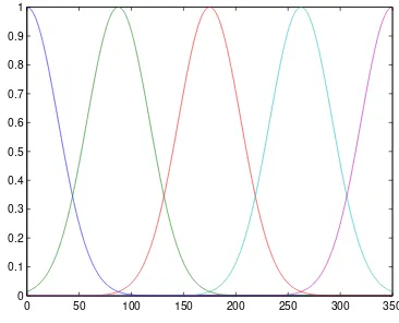
Fig. 4. Gaussian Fuzzy Sets of the Linguistic Variablex3
Fig. 5. Direct Fuzzy Adaptive Control Structure
our study uses the sixth-order polynomial torque coefficient which captures all operating regions.
The fuzzy model uˆ(x) used to approximate the control
u∗(x)is chosen as Takagi-Sugeno model which has inference rules in the form
Ifx1 is A1i andx2 is A2i and x3 is A3i thenuˆ(x) = θui, wherex1,x2, andx3 are state variables;A1i,A2i, andA3i are fuzzy sets of linguistic variables describing x1,x2, and x3 respectively at the ith rule. The forms and number of
fuzzy sets for linguistic variables are chosen based on trial and error basis. In this system fuzzy set forms were chosen as Gaussian and there are five fuzzy sets for each linguistic variable as shown in Fig. 4. Consequently there are total 125 rules.
The approximate fuzzy system in (30) is
ˆ
u(x) =θuTξu(x),
where
θu = θu1θu2...θu125
T
, (48)
ξu(x) =
ξu1(x)ξu2(x)...ξu125(x)
T
, (49)
ξui =
µA1i(x1).µA2i(x2).µA3i(x3)
P125
i=1µA1i(x1).µA2i(x2).µA3i(x3) , (50)
whereξui is the regressor at theith rule.
The direct fuzzy adaptive control structure is shown in Fig. 5 where the adaptive controller is given in (30) with the adaptive law given in (42), and the supervisory controller is given in (46).
V. SIMULATIONRESULTS
[image:4.595.334.517.62.210.2]TABLE I SIMULATIONDATA
Wind Rotor Drive Train PMSG R = 2.5 m i = 7 p = 3,Rs= 3.3 Ω
ρ= 1.25kg/m3 η= 1 L
d= 0.04156H
Jh= 0.0552kg.m2 Lq= 0.04156H
Ls= 0.08H Φm= 0.4382W b
0 10 20 30 40 50
5 5.5 6 6.5 7 7.5 8 8.5 9 9.5
Time(s)
Wind Speed (m/s)
Fig. 6. Simulation Wind Speed Profile
0 10 20 30 40 50
0 5 10 15 20 25 30
Time (s)
[image:5.595.68.390.42.641.2]Speed (rad/s) Optimal Generator Speed Direct Fuzzy Adaptive Control Feedback Linearization Control
Fig. 7. Output Reference Tracking
CPmax = 0.478 and the optimal tip-speed ratio λ
∗ = 7.
Other system parameters are given Table I. Lower and upper bounds in assumption 2, 3, and 4 are δ¯u = 0.001, β = 1, and βv = 30. The nonlinear PMSG-based WECS has the relative degree r= 2, so parameters for the error dynamics are chosen as γ = 15 and k1 = 5. The control input is
set bounded as 0 < u ≤ 100. The stochastic wind profile is shown in Fig. 6. Control performances of both Direct Fuzzy Adaptive Control (DFAC) proposed in this paper and Feedback Linearization Control (FLC) proposed in [5] are compared in parallel.
Regarding the output tracking performance, Fig. 7 and 8 show both DFAC and FLC track the output reference
0 10 20 30 40 50
0 10 20 30 40 50 60 70 80 90 100
Time (s)
Load Resistance (Ohm)
Direct Fuzzy Adaptive Control Feedback Linearization Control
Fig. 8. Control Inputs
0 10 20 30 40 50
0 1 2 3 4 5 6 7 8 9 10
Time (s)
Tracking Error Square
[image:5.595.155.532.61.709.2]Direct Fuzzy Adaptive Control Feedback Linearization Control
Fig. 9. Tracking Errors
0 10 20 30 40 50
0 0.05 0.1 0.15 0.2 0.25 0.3 0.35 0.4 0.45 0.5
Time (s)
Power Coefficient
Direct Fuzzy Adaptive Control Feedback Linearization Control
Fig. 10. Optimal Power Coefficient Maintenance
[image:5.595.311.542.68.485.2]0 10 20 30 40 50 0
1 2 3 4 5 6 7 8
Time (s)
The Tip−speed Ratio
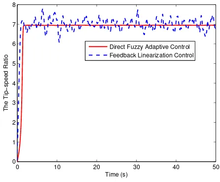
[image:6.595.63.286.63.247.2]Direct Fuzzy Adaptive Control Feedback Linearization Control
Fig. 11. Optimal Tip-speed Ratio Maintenance
Regarding the power conversion efficiency, two important factors representing the optimal power extraction are the power coefficient maintenance and tip-speed ratio mainte-nance under wind speed fluctuations. Fig. 10 and 11 prove the DFAC better than the FLC in optimizing the power conversion. It is obviously observed from those figures that the DFAC stays constantly steady at the optimal power coefficient and tip-speed ratio values after the transient time. Meanwhile, the FLC keeps oscillating around optimal values.
VI. DISCUSSION ANDCONCLUSION
The simulation results show that the proposed DFAC is very good in dealing with the time-varying, nonlinear nature of WECS. The DFAC was also proven more effective than the FLC regarding the control performance and power capture. However, the design of DFAC requires certain assumptions to be met as stated in Section III which are not always satisfied in practice. For example, it is hard to find lower and upper bounds of the nonlinear functionβ(x)
and structural error δu(x). These values were found based on the system physical features combined with the trial and error method in this paper.
Another important note is that both DFAC and FLC require all states to be accessible. As we know that system states are not available sometime and/or somewhere; consequently the DFAC and FLC are not applicable in those situations. Therefore, an extension of this study would be construct-ing a nonlinear observer to estimate unavailable states and integrating the nonlinear observer into the DFAC scheme.
REFERENCES
[1] M. Stiebler, Wind Energy Systems for Electric Power Generation. Springer-Verlag, 2008.
[2] C. Abbey, K. Strunz, and G. Joos, “A knowledge-based approach for control of two-level energy storage for wind energy systems,”Energy Conversion, IEEE Transactions on, vol. 24, no. 2, pp. 539 –547, June 2009.
[3] S. Teleke, M. Baran, A. Huang, S. Bhattacharya, and L. Anderson, “Control strategies for battery energy storage for wind farm dispatch-ing,”Energy Conversion, IEEE Transactions on, vol. 24, no. 3, pp. 725 –732, Sept. 2009.
[4] S. Teleke, M. Baran, S. Bhattacharya, and A. Huang, “Optimal control of battery energy storage for wind farm dispatching,”Energy Conver-sion, IEEE Transactions on, vol. 25, no. 3, pp. 787 –794, Sept. 2010.
[5] I. Munteanu, A. Bratcu, N. Cutuluslis, and E. Ceanga,Optimal Control of Wind Energy Systems: Toward a Global Approach. Springer, 2008. [6] K. Astrom and T. Hagglund,Adaptive Control. Dover Publications
Inc., Mineola, N.Y., U.S., 2008, second Edition.
[7] W. Dinghui, X. Lili, and J. Zhicheng, “Fuzzy adaptive control for wind energy conversion system based on model reference,” inControl and Decision Conference, 2009. CCDC ’09. Chinese, Jun. 2009, pp. 1783 –1787.
[8] J. Qi and Y. Liu, “PID control in adjustable-pitch wind turbine system based on fuzzy control,” in Industrial Mechatronics and Automation (ICIMA), 2010 2nd International Conference on, vol. 2, May 2010, pp. 341 –344.
[9] X. Yao, H. Wen, Y. Deng, and Z. Zhang, “Research on rotor excitation neural network PID control of variable speed constant frequency wind turbine,” inElectrical Machines and Systems, 2007. ICEMS. Interna-tional Conference on, Oct. 2007, pp. 560 –565.
[10] X. Yao, X. Su, and L. Tian, “Wind turbine control strategy at lower wind velocity based on neural network PID control,” in Intelligent Systems and Applications, 2009. ISA 2009. International Workshop on, May. 2009, pp. 1 –5.
[11] ——, “Pitch angle control of variable pitch wind turbines based on neural network PID,” inIndustrial Electronics and Applications, 2009. ICIEA 2009. 4th IEEE Conference on, May. 2009, pp. 3235 –3239. [12] Z. Xing, Q. Li, X. Su, and H. Guo, “Application of BP neural
network for wind turbines,” inIntelligent Computation Technology and Automation, 2009. ICICTA ’09. Second International Conference on, vol. 1, Oct. 2009, pp. 42 –44.
[13] L.-X. Wang,A Course in Fuzzy Systems and Control. Prentice-Hall. Inc., Upper Saddle River, New Jersey, U.S., 1996.
[14] H. T. Huynh,Intelligent Control Systems. Ho Chi Minh National University Press, 2006.
[15] H. Khalil,Nonlinear Systems,2ndEdition. Prentice-Hall. Inc., Upper