Evolutionary GRSA for Protein Structure Prediction

Received Jan 29, 2016 / Accepted Aug 21, 2016

Editorial Académica Dragón Azteca (EDITADA.ORG)

Evolutionary GRSA for Protein Structure Prediction

Fanny Gabriela Maldonado-Nava

_{, Juan Frausto-Solís}

_{, Juan Paulo Sánchez-Hernández}

_{, Juan Javier}

González-Barbosa

_{, Ernesto Liñán-García}

_{, Guadalupe Castilla Valdez}

1

_{Tecnológico Nacional de México, Instituto Tecnológico de Ciudad Madero}

Universidad Politécnica del Estado de Morelos

3

_{Universidad Autónoma de Coahuila. Facultad de Sistemas.}

E-mail:

[email protected], [email protected], [email protected],

[email protected], [email protected]

Abstract. Protein folding problem (PFP) is a challenge in some areas, such as molecular biology, computational biology, combinatorial optimization, and computer science. This is due to the large number of conformational structures that a protein can take from its primary structure to the native structure (NS). The aim of PFP is to find the NS of a protein target sequence. In general, the NS which has the lowest Gibbs energy or an energy close to it. In this paper, a Simulated Annealing like algorithm is presented, using the Golden Ratio search strategy and evolutionary techniques for PFP in small peptides. This method looks for the NS using only the protein's amino acid sequence, and determines the three-dimensional structure with the minimum energy or a close value of it.

Keywords: Protein Structure Prediction, GRSA, Evolutionary algorithms.

1. Introduction

Proteins are molecules made of amino acids. They play a central role in biological processes. For example, proteins transport molecules such as oxygen (hemoglobin), also they are involved in the immune system (antibodies), and provide support in our bodies (collagen and elastin). The atoms of a protein are linked in a three-dimensional structure where Gibbs free energy is the lowest [1]. Is in this structure in which a protein can perform its biological function in our body. PFP is an NP-hard problem that consists of finding the three-dimensional structure of a protein; this structure is known as Native Structure (NS) and is characterized by the lowest energy in the last configuration of amino acids’ atoms [2][1][3]. A protein can take a high number of different conformational structures from its amino acids sequence (primary structure) to its NS, therefore, the total number of possible conformations is an exponential function of the total number of degrees of freedom in the amino acid chain. The natural process in which a protein gets to its native state is not understood at all, because in nature a protein does not explore all its possible states. So, the protein takes an unknown path to its native structure [4]. The importance of PFP lies in the fact that certain diseases as Alzheimer, Parkinson, Prion, and Tauopathy, are related to the incorrect folding of some proteins [5], this is the main reason why it is important to understand the protein folding process, because this may lead to manipulation of proteins to prevent or find the cure for some illnesses.

76

Due to the complexity of the problem and the long time that takes to analyze all that possible conformations, and that even for a small protein molecule the high dimensionality of the search space makes the problem intractable [4], only a tiny portion of protein sequences have experimentally solved three-dimensional structures. This fact had motivated further research in Computational Protein Structure Prediction Methods. Different computational approaches for finding the three-dimensional structure have been proposed. Algorithms are based on these strategies for solving protein folding problem, these algorithms search structures on a huge space of possible solutions. These methods can obtain several structures very close to the native structure. These computational strategies can be classified into 3 categories: (a) ab initio, (b) homology, and (c) threading [7]. Homology and threading methods use protein information looking for finding a solution of the problem, in contrast, ab initio

uses only the amino acid sequence without additional structural information. Anfinsen (Nobel Prize in Chemistry, 1972) shows that only ab initio can solve PFP [1]. Ab initio is an interesting strategy for the next reasons: a) a lot of proteins do not have any homology with other proteins which native structure is known; b) the other strategies do not give information about why a protein adopts a certain structure; and c) even though, some proteins show high resemblance to other proteins, they adopt structures completely different [8]. On the contrary, the bases of ab initio come from physical concepts based on energy functions [9], which can be model as an optimization problem. As a result, only predictions made with ab initio can be fully reliable. The algorithm proposed in this work belongs to the ab initio strategy.

For solving PFP, some heuristics methods have been used, most common are simulated annealing (SA), genetic algorithms (GA), ant colony optimization (ACO), tabu search (TS), and other heuristics. The most successful methods for finding the PFP solution are heuristics based on Simulated Annealing (SA), and Monte Carlo method; these successful methods are usually hybridized with other heuristics and strategies [10]. However, simulating the folding of a protein from a stretched configuration to its native structure remains a challenge [11], and the scientific community is working on more powerful algorithms, and trying to solve the question related to Levintal´s Paradox: how nature does protein folding? [4]. To answer this unsolved question is important because PFP is an NP-Hard problem, but nature uses only some seconds or even nanoseconds for any protein folding process.

To generate high-quality solutions for PFP, new and more efficient SA algorithms have been designed; Golden Ratio Simulated Annealing (GRSA) is one of these algorithms [12]; this algorithm has shown to be very efficient for small proteins as Met-enkephalin, C-Peptide, 1EOG, 1ENH, and 1BDD. GRSA uses several strategies for finding the best solution of PFP. In GRSA, SA parameters are tuned with an analytical method, uses a heuristic technique for dividing the search space into sections, it has a phase which detects the thermal equilibrium by a least squares method, and a reheat strategy to escape from local optima. In this paper, we propose a hybrid algorithm based on GRSA and evolutionary techniques. The performance of the new algorithm named EGRSA (Evolutionary Golden Ratio Simulated Annealing) is compared with GRSA using the pentapeptide Met-enkephalin. The experimentation discussed in the paper shows that the new algorithm finds similar results to the those reported by GRSA. This is important because PFP can be solved for bigger proteins.

This paper is organized as follows: in section 2, Protein Folding Problem is described. Section 3, describes the simulated annealing algorithm and techniques used in the GRSA hybridization. Section 4, describes the analytical tuning method used by GRSA and EGRA. In section 5, EGRSA is presented. Finally, in section 6 the results obtained by EGRSA are shown and compared with those obtained by GRSA.

2. Protein Folding Problem

Protein folding problem is the process of finding the three-dimensional native structure of a protein, in this conformation the protein fulfills its biological function. Find the NS among all the possible conformations of a protein is an enormous challenge because the space of possible conformations is extremely large [2].

For practical purposes, PFP can be defined using the free energy 𝑓(𝝈) of the amino acids set, where 𝝈 is a vector of the 𝑚

dihedral angles of the amino acids; that is 𝝈 = {𝜎1, 𝜎2, 𝜎3, … , 𝜎𝑚}. More precisely, PFP consists of finding the minimum free energy 𝑓∗_(𝝈∗_{). Then, PFP is definedas follows:}

77

 Find the native structure of the protein, such that 𝑓∗(𝝈∗) represents the minimum energy value, where the optimal solution 𝝈∗_{= {𝜎}

1∗, 𝜎2∗, 𝜎3∗, … , 𝜎𝑚∗} defines the best three-dimensional configuration. The PFP variables are the set 𝝈 of dihedral angles.

The atoms of a protein are represented in three-dimensional Cartesian coordinates. There are four types of torsion angles or dihedral angles:

 The angle between the amino group and the alpha carbon is referred as Phi (𝜙). This angle represents the angle between the amino group (or 𝑁𝐻2) of the amino acid 𝑖, and the alpha Carbon 𝐶𝑖 in the sequence; it represents the bond angle between the 𝑁𝑖 atom of amino group and the alpha carbon (𝛼𝐶𝑖).

 The dihedral angle between the alpha carbon and the carboxyl group is referred as Psi (𝜓 ). Psi represents the angle between the carboxyl (𝐶𝑂𝑂𝐻𝑖) group of the amino acid 𝑖, and the alpha carbon 𝑖 (𝐶𝑖) of the same amino acid. Psi measures the angle of the covalent bond between the 𝐶𝑖 of the carboxyl group, and the alpha carbon (𝛼𝐶𝑖).

 The omega angle (𝜔) is defined for each two consecutive amino acids; it is the angle of the covalent bond between the atom 𝑁𝑖 of amino acid 𝑖, and carbon 𝐶(𝑖−1) of the carboxyl group of the amino acid (𝑖 − 1).

 And, finally each Chi angle (

𝜒

The determination of the value for these four angles for each of the amino acids that make up the protein sequence, constitute the variables of the problem.

The protein’s energy depends on the interaction among their atoms. And this energy is affected by the position of atoms, torsion angles and distance among atoms. To measure the energy of a protein, force fields are used; these include many interactions among atoms affecting different energies [13]. A force field includes terms associated with the bond interactions, and terms associated with no-bond interactions. The bond interactions are associated with chemical bonds, for example hydrogen bond interactions. The no-bond interactions include interaction between atoms that are not directly joined by chemical bonds; for example, electrostatic and Van der Waals interactions. Some of the most popular and successful software systems for calculating force fields are CHARMM [14], AMBER [15], ECEPP/2 and ECEPP/3 [16]. In this paper ECEPP/2 force field is used [17].

ECEPP is a relatively simple force field based on rigid geometry (i.e., constant bond angles and lengths), with conformations thus defined solely by the backbone and side chain dihedral angles. In ECEPP/2 the potential energy is given by the sum of the electrostatic term 𝐸𝑒𝑙𝑒𝑐𝑡𝑟𝑜𝑠𝑡𝑎𝑡𝑖𝑐, Lennard-Jones term 𝐸𝐿𝐽, and hydrogen-bond term 𝐸𝐻𝐵 for all pairs of atoms in the peptide together with the torsion term 𝐸𝑡𝑜𝑟 for all torsion angles [18]:

𝐸𝑏𝑜𝑛𝑑𝑒𝑑= 𝐸𝑒𝑙𝑒𝑐𝑡𝑟𝑜𝑠𝑡𝑎𝑡𝑖𝑐+ 𝐸𝐿𝐽+ 𝐸𝐻𝐵+ 𝐸𝑡𝑜𝑟 (1)

These terms in equation (1) are expressed in equation (2) through which energy function ECEPP/2 minimize the energy [18].

𝐸𝑡𝑜𝑡𝑎𝑙= ∑ (

𝐴𝑖𝑗

𝑟12 𝑖𝑗

− 𝐵𝑖𝑗 𝑟6

𝑖𝑗

) +

𝑗>𝑖

332 ∑𝑞𝑖𝑞𝑗 𝜀𝑟𝑖𝑗

𝑗>𝑖

+ ∑ ( 𝐶𝑖𝑗 𝑟12

𝑖𝑗

− 𝐷𝑖𝑗 𝑟10

𝑖𝑗

)

𝑗>𝑖

+ ∑ 𝑈𝑛(1 ± cos(𝑘𝑛𝜑𝑛)) 𝑛

(2)

Where:

- 𝑟𝑖𝑗is the distance in Å between the atoms 𝑖 and 𝑗.

- 𝐴𝑖𝑗, 𝐵𝑖𝑗, 𝐶𝑖𝑗 and 𝐷𝑖𝑗 are the parameters of the empirical potentials. - 𝑞𝑖and𝑞𝑗are the partial charges on the atoms 𝑖 and 𝑗, respectively. - 𝜀 is the dielectric constant which is usually set to 𝜀 = 2.

78

3. Golden Ratio Simulated Annealing

Simulated Annealing (SA) algorithm was proposed by Kirkpatrick, which applies the Metropolis algorithm to minimization problems [19]. SA represents a thermodynamic process where the metal passes through a thermodynamic phase called annealing. Simulated annealing is a procedure that introduces a random phase in the acceptance of movements, such that if the movement produces an improvement in the solution, then it is accepted; on the contrary, if the movement leads to a worse solution, a criterion based on Boltzmann’s probability is applied in order to decide whether the solution is accepted or not. SA begins generating an initial solution, which is set as the current solution. Classical simulated annealing consists of two cycles; an external cycle that is controlled by a temperature parameter, which varies temperature from a high temperature to a close to zero final temperature; the temperature is very slowly reduced using a cooling function. Inside the temperature cycle the Metropolis cycle is executed, inside this inner cycle a new solution is generated by modifying the previous solution by a perturbation function. After Metropolis cycle is completed, the value of the temperature is updated. This procedure can be observed in the algorithm 1.

Algorithm 1. Classical Simulated Annealing

1: SA (𝑇𝑖, 𝑇𝑓𝑝, 𝑇𝑓, 𝛼) 2: 𝑇𝑘= 𝑇𝑖

3: 𝑆𝑖= 𝑔𝑒𝑛𝑒𝑟𝑎𝑡𝑒𝑆𝑜𝑙𝑢𝑡𝑖𝑜𝑛() 4: while𝑇𝑘≥ 𝑇𝑓do

5: while𝑀𝑒𝑡𝑟𝑜𝑝𝑜𝑙𝑖𝑠do

6: 𝑆𝑗 = 𝑝𝑒𝑟𝑡𝑢𝑟𝑏𝑎𝑡𝑖𝑜𝑛(𝑆𝑖) 7: ∆𝐸 = 𝐸(𝑆𝑗) − 𝐸(𝑆𝑖) 8: if∆𝐸 ≤ 0then

9: 𝑆𝑖 = 𝑆𝑗

10: else if𝑒−∆𝐸/𝑇𝑖 _{< 𝑟𝑎𝑛𝑑𝑜𝑚[0; 1)then}

11: 𝑆𝑖 = 𝑆𝑗 12: end

13: end

14: 𝑇𝑘+1 = 𝛼 ∗ 𝑇𝑘 15: end

16: end

Simulated annealing has been used for solving PFP as mentioned earlier. However, the classic SA may take a lot of time and can be trapped on local minima. To improve the quality of the results obtained by SA, some heuristics and techniques can be used, such as the Golden Ratio search technique. Golden Ratio (GR) is an irrational number used in antiquity to design architectural masterpieces, and is represented by the letter Φ. GR is applied as a search strategy to find the maximum or minimum a function with some efficacy [20]. This strategy is based on eliminating a region, at each stage, of the interval in which the minimum or maximum is comprised and when the possible region is small enough the search ends. These techniques use a constant relationship to divide the interval into segments and in this way, will be reduced the search space.

We can find a GR extension, that is an hybridization of GR and simulated annealing, named GRSA (Golden Ratio Simulated Annealing) algorithm, which has been applied for NP-hard problems such as Scheduling [21] and SAT [22]. Recently GRSA was successfully applied to the PFP, obtaining very good quality solutions for some peptides [12]. However, it is necessary to improve the quality of solutions obtained by GRSA to increase its applicability. GRSA for PFP hybridize Golden Ratio and Simulated Annealing in an algorithm that divides the solution space into sections [12]. This algorithm uses three main strategies: firstly, temperature parameters are tuned with an analytical-experimental approach; secondly, a special phase which detects the thermal equilibrium by a least squares method; and a reheat strategy to escape from local optima is applied.

79

begins where the value of the parameter 𝛼 is updated and another 𝑇𝑓𝑝 is recalculated. This procedure continues until the number of cuts (𝑇𝑓𝑝𝑛) is reached, the last phase is executed until the final temperature is reached. Other strategy we can find in GRSA is a stop criterion (SC), which is implemented when the algorithm at low temperatures no longer improves its quality. To determine the stop condition, the least squares method is applied, this method uses a linear equation 𝐸(𝐼) = 𝑚𝐼 + 𝑏, where 𝐸(𝐼)

is the set of energies for every 𝐼 metropolis cycle, 𝑚 is the slope and 𝑏 is the interceptor. The equilibrium is almost reached when 𝑚 is close to zero [14]. If 𝑚 is close to zero, GRSA is finished. In order to improve its quality, in the GRSA algorithm, a reheat strategy (RH) was implemented, which is applied in two phases: a) at the end of the last GR section and b) when the equilibrium is detected [12].

4. Analytical tuning

For a better performance of the Simulated annealing algorithms, parameters must be tuned. More efficiency and efficacy of the Simulated Annealing algorithm can be achieved using the best values for some parameters of the cooling scheme. The cooling scheme includes the cooling function, the initial and final temperatures, and the length of the Markov chain.

The initial temperature of the algorithm should allow the acceptance of all possible transitions and the free movement in the solution space. When the temperature is very high, almost any solution is acceptable even if it is worse than the current one. When the temperature is very small, it only accepts solutions that are better than the current one. If the initial temperature is too high, a lot of time can be wasted in the first few cycles, and if it is very low, the probability of being trapped in a local optimum is very high. However, if the final temperature is very high, the probability of being trapped in a local optimum is very high. If the temperature is very low, probably the search process will be very exhaustive and will consume a lot of time. Therefore, a good choice of the initial and final temperature is of great importance to achieve a good performance of the SA.

Simulated Annealing requires a well-defined neighborhood structure and other parameters as initial and final temperatures. To determine these parameters, an analytical tuning method was applied. This method is described as follows:

The calculation of the initial temperature 𝑇𝑖 is based on the accepting probability 𝑃𝐴(𝑆𝑗) of one proposed solution (𝑆𝑗) and the maximum cost deterioration of the objective function named ∆𝑍𝑉𝑚𝑎𝑥. ∆𝑍𝑉𝑚𝑎𝑥 gives the maximum deterioration that may be produced during the execution of the algorithm, so the way of making sure that ∆𝑍𝑉𝑚𝑎𝑥 be accepted, at the initial temperature

𝑇𝑖. At the beginning 𝑃𝐴 is close to 1; 𝑃𝐴(∆𝑍𝑖𝑗) ≈ 1, and the temperature is extremely high, almost any solution is accepted at this temperature. When the process is ending, the acceptance probability is too low (𝑃𝐴(∆𝑍𝑖𝑗) ≈ 0). The initial temperature 𝑇𝑖 is calculated as follows:

𝑇𝑖= −

∆𝑍𝑉𝑚𝑎𝑥

ln(𝑃𝐴(∆𝑍𝑉𝑚𝑎𝑥 ))

(3)

∆𝑍𝑉𝑚𝑖𝑛 establishes the minimum deterioration that can be produced during the execution of the algorithm. In a similar way that for 𝑇𝑖 temperature, the final temperature 𝑇𝑓 is setting by the next equation:

𝑇𝑓= −

∆𝑍𝑉𝑚𝑖𝑛

ln(𝑃𝐴(∆𝑍𝑉𝑚𝑖𝑛 ))

(4)

Not only initial and final temperatures are calculated with the analytical tuning, as the same way does the Metropolis cycle length. Analytical method determines the Metropolis cycle length 𝐿𝑘 with a Markov model.

80

𝑇𝑘+1= 𝛼𝑇𝑘 (5)

where α is normally in the range of 0.7 ≤ α ≤ 0.99.

The length of each Markov chain must be incremented at any temperature cycle in a similar but in inverse way that 𝑇𝑘 is decremented. That means, 𝐿𝑘 must be incremented until 𝐿𝑚𝑎𝑥 is reached at 𝑇𝑓 by applying an increment Markov chain factor 𝛽. The cooling function given by (5) is applied many times until the final temperature 𝑇𝑓 is reached. Because Metropolis cycle is finished when the stochastic equilibrium is reached, it can be also modeled as a Markov Chain as follows:

𝐿𝑘+1= 𝛽𝐿𝑘 (6)

𝐿𝑘 represents the length of the current Markov chain at a given temperature, that means the number of iterations of the Metropolis cycle for a 𝑘 temperature. So, 𝐿𝑘+1 represents the length of the next Markov chain. In this Markov Model, 𝛽 represents an increment of the number of iterations in the next Metropolis cycle.

The cooling function is applied repeatedly until 𝑇𝑘 = 𝑇𝑓 we get:

𝑇1= 𝛼𝑇1

𝑇2= 𝛼𝑇1= 𝛼2𝑇1

𝑇3= 𝛼𝑇2= 𝛼3𝑇1

⋮

𝑇𝑛= 𝛼𝑇𝑛−1= 𝛼𝑛𝑇1 (7)

Therefore, we can see that if we know the initial (𝑇1) and final (𝑇𝑓) temperatures and the cooling coefficient (𝛼), the number of times that the Metropolis cycle is executed can be calculated as:

ln 𝑇𝑓 = 𝑛 ln 𝛼 + ln 𝑇1

𝑛 =ln 𝑇𝑓− ln 𝑇1

ln 𝛼 (8)

In a similar way, applying systematically 𝐿𝑘+1= 𝛽𝐿𝑘 we get:

𝐿1= 𝛽𝐿1

𝐿2= 𝛽𝐿1= 𝛽2𝐿1

𝐿3= 𝛽𝐿2= 𝛽3𝐿1

⋮

𝐿𝑛= 𝛽𝐿𝑛−1= 𝛽𝑛𝐿1

𝐿𝑚𝑎𝑥 = 𝛽𝑛𝐿1 (9)

𝛽 = exp (ln 𝐿𝑚𝑎𝑥− ln 𝐿1

𝑛 ) (10)

81

5. Evolutionary Golden Ratio Simulated Annealing

In this work, we propose a GRSA hybridization [12] with evolutionary techniques for solving PFP. As is well known, evolutionary algorithms, are a neo-Darwinian approach to species evolution based on the idea that individuals who have a better adaptation to the environment have a higher probability of living longer, and generate offspring that inherit their characteristics. On the other hand, individuals with poorer adaptation to the environment are less probably to survive, to be offspring and more probably to become extinct.

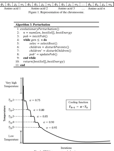
EGRSA is presented in algorithm 2. The difference between a classic SA and EGRSA is the perturbation and the cooling scheme, in EGRSA to get a new solution (perturbation), an evolutionary strategy is used (line 7). The cooling scheme is calculated in lines 15-20. When the current temperature reaches 𝑇𝑓𝑝 (previously calculated using golden number Φ), the 𝛼 parameter is updated and the next 𝑇𝑓𝑝 value is computed. This allows a dynamic behavior of the cooling scheme (in Fig. 1 this behavior can be observed).

Algorithm 2. EGRSA

1: SA (𝑇𝑖, 𝑇𝑓𝑝, 𝑇𝑓, E, S, 𝛼) 2: 𝑇𝑘= 𝑇𝑖

3: 𝑆𝑖= 𝑔𝑒𝑛𝑒𝑟𝑎𝑡𝑒𝑆𝑜𝑙𝑢𝑡𝑖𝑜𝑛() 4: while𝑇𝑘≥ 𝑇𝑓do

5: 𝑇𝑓𝑝= 𝑇𝑓𝑝∗ Φ 6: while𝑀𝑒𝑡𝑟𝑜𝑝𝑜𝑙𝑖𝑠do

7: 𝑆𝑗 = 𝑒𝑣𝑜𝑙𝑢𝑡𝑖𝑜𝑛𝑎𝑟𝑦𝑃𝑒𝑟𝑡𝑢𝑟𝑏𝑎𝑡𝑖𝑜𝑛(𝑆𝑖) 8: ∆𝐸 = 𝐸(𝑆𝑗) − 𝐸(𝑆𝑖)

9: if∆𝐸 ≤ 0then

10: 𝑆𝑖 = 𝑆𝑗

11: else if𝑒−∆𝐸/𝑇𝑖 _{< 𝑟𝑎𝑛𝑑𝑜𝑚[0; 1)then}

12: 𝑆𝑖 = 𝑆𝑗 13: end if

14: end while

15: if𝑇𝑘 ≤ 𝑇𝑓𝑝then 16: 𝛼 = 𝛼𝑛𝑒𝑤 17: 𝑇𝑘+1 = 𝛼 ∗ 𝑇𝑘 18: else

19: 𝑇𝑘+1 = 𝛼 ∗ 𝑇𝑘 20: end if

21: end while

22: end

82

𝜙1 𝜓1 𝜒1 𝜔1 𝜙2 𝜓2 𝜒2 𝜔2 𝜙3 𝜓3 𝜒3 𝜔3 … 𝜙𝑛 𝜓𝑛 𝜒𝑛 𝜔𝑛 Amino acid 1 Amino acid 2 Amino acid 3 … Amino acid 𝑛

Figure 1. Representation of the chromosome.

Algorithm 3. Perturbation

1: 𝑒𝑣𝑜𝑙𝑢𝑡𝑖𝑜𝑛𝑎𝑟𝑦𝑃𝑒𝑟𝑡𝑢𝑟𝑏𝑎𝑡𝑖𝑜𝑛()

2: 𝑛 = 𝑛𝑢𝑚𝐺𝑒𝑛, 𝑏𝑒𝑠𝑡𝑆𝑜𝑙[], 𝑏𝑒𝑠𝑡𝐸𝑛𝑒𝑟𝑔𝑦

3: 𝑝𝑜𝑏 = 𝑖𝑛𝑖𝑐𝑖𝑡𝑃𝑜𝑏()

4: while𝑔𝑒𝑛 ≤ 𝑛do

5: 𝑠𝑒𝑙𝑒𝑐 = 𝑠𝑒𝑙𝑒𝑐𝑡𝐵𝑒𝑠𝑡()

6: 𝑐ℎ𝑖𝑙𝑑𝑟𝑒𝑛 = 𝑑𝑖𝑠𝑡𝑢𝑟𝑏𝑃𝑎𝑟𝑒𝑛𝑡𝑠()

7: 𝑐ℎ𝑖𝑙𝑑𝑟𝑒𝑛∗_{= 𝑑𝑖𝑠𝑡𝑢𝑟𝑏𝐶ℎ𝑖𝑙𝑑𝑟𝑒𝑛()} 8: 𝑝𝑜𝑏∗_{= 𝑢𝑝𝑑𝑎𝑡𝑒𝑃𝑜𝑏()}

9: end while

10: 𝑟𝑒𝑡𝑢𝑟𝑛(𝑏𝑒𝑠𝑡𝑆𝑜𝑙[], 𝑏𝑒𝑠𝑡𝐸𝑛𝑒𝑟𝑔𝑦)

11: end

Fig. 1. GRSA temperature behavior.

6. Implementation and Results

83

In this paper the energy function ECEPP/2 implemented in the software package SMMP is used [17]. ECEPP/2 was chosen because the state of the art research work used for comparative purposes applies this force field, and because for ECEPP/2 the Met-enkephalin lowest energy conformation is known [26][27][28]. The initial and final temperatures of the algorithm were tuned with an analytical method [10] described in section 4. In this implementation, five GR sections, a stop criterion, and reheat strategy are used in order to compare results with GRSA using the same strategies, and to observe the differences between the original perturbation [12] and the evolutive perturbation used in EGRSA.

EGRSA was executed 30 times to validate the algorithm results. This experimentation was carried out in a personal computer, with the following characteristics: Intel Core i5 3210M processor at 2.50 GHz, memory 6.0 GB, and Windows 7 Professional 64-bit operative system, and the best solution was obtained.

The best energies (expressed in kcal/mol) obtained by EGRSA with the five GR sections and the stop criterion (SC) are compared to those obtained with GRSA and the same strategies, these results are shown in Table 1. We can observe in table 1 that in this implementation the best energy was obtained by EGRSA with the stop criterion and five golden sections, the energy obtained was -10.6925 kcal/mol. While GRSA, using the same strategies obtained -10.6006 kcal/mol.

Table 1. Met-enkephalin results with GRSACP and EGRSACP.

Number of GR Sections GRSASC EGRSASC

GR 1 -10.4528 -9.2848

GR 2 -10.1119 -10.0529

GR 3 -10.5314 -10.5846

GR 4 -10.6006 -10.3601

GR 5 -10.1540 -10.6925

A second implementation of EGRSA was tested, but in this case the reheat strategy (RH) was included in together with five GR sections and the stop criterion (SC). Best energies for Met-enkephalin obtained by EGRSA (five GR section, a stop criterion and reheat strategy) are compared to those obtained by GRSA (five GR sections, stop criterion and reheat strategy) and are shown in table 2. We can see in table 2, that the best results with these strategies were obtained by GRSA using one golden section, the minimum energy is -10.6360 kcal/mol. While best energy obtained by EGRSA was -10.1562 kcal/mol.

Table 2. Met-enkephalin results with GRSARHCP and EGRSARHCP.

Number of GR sections GRSARHCP EGRSARHCP

GR 1 -10.6360 -10.0812

GR 2 -10.3443 -10.1201

GR 3 -10.5174 -9.8942

GR 4 -10.3552 -10.1562

GR 5 -10.1838 -9.5018

84

Best solutions quality found by EGRSA for Met-Enkephalin are shown in table 3. We can observe that the RMSD and TM score for the best solution of EGRSA are 0.19 and 0.52416, respectively. Consequently, the energy of -10.6925 kcal/mol is a correct solution. Furthermore, the RMSD and TM-Score indicate that the configuration presents a good alignment to the native structure. Notice, that even the second best result (with an energy value of -10.1562 kcal/mol) is an acceptable solution; this is because the RMSD and TM-score values are into the acceptable criteria.

Table 3. Best energy, RMSD and TM-Score for Met-Enkephalin.

Energy value

(kcal/mol) Strategy

Golden

section RMSD TM-Score

-10.6925 Stop criterion 5 GR 0.19 0.52416

-10.1562 Stop criterion

Reheat 4 GR 0.36 0.39550

For Met-enkephalin the best results reported in literature using the force field ECEPP/2 are -10.72 kcal/mol (𝜔 angle fixed to 180°) [17] and -12.90 kcal/mol (𝜔 angle variable) [29]. For classic simulated annealing the best reported result is -5 kcal/mol [29]. Notice that the best energy found by EGRSA of -10.6925 kcal/mol is very close of the native structure and the difference is less than one percent (barely 0.25 %).

7. Conclusions

In this work a simulated annealing algorithm hybridized with Golden Ratio strategy and an evolutionary algorithm applied to the protein folding problem was presented. Experimentation was performed with Met-Enkephalin, which is usually used as a benchmark. Results obtained by this algorithm were compared with results obtained by GRSA and three strategies (GR sections, stop criterion and reheat). As we can see in section 6, two implementations were tested: an implementation of EGRSA using five golden sections and a stop criterion, and a second implementation using additionally a reheat strategy.

For the first implementation of EGRSA algorithm, results show that it had better performance than the original GRSA and very close to the native structure. In fact, the solution found by the proposed algorithm is practically the same corresponding to the NS. The measures used related to the quality of PFP algorithms indicate a very good performance of the proposed algorithm. As a future work, new research should be developed in order to evaluate bigger peptides and proteins.

Acknowledgements

The authors would like to acknowledge with appreciation and gratitude to CONACYT. Also, acknowledge to Laboratorio Nacional de Tecnologías de la Información (LaNTI) of the Instituto Tecnológico de Ciudad Madero for the access to the cluster. Fanny Gabriela Maldonado-Nava would like to thank CONACYT for the support in the project 429028.

References

[1] C. B. Anfinsen, “Principles that Govern the Folding of Protein Chains,” Science (80-. )., vol. 181, no. 4096, pp. 223– 230, Jul. 1973.

[2] J. T. Ngo, J. Marks, and M. Karplus, “Computational Complexity, Protein Structure Prediction, and the Levinthal Paradox,” in The Protein Folding Problem and Tertiary Structure Prediction, Boston, MA: Birkhäuser Boston, 1994, pp. 433–506.

[3] P. Crescenzi, D. Goldman, C. Papadimitriou, A. Piccolboni, and M. Yannakakis, “On the Complexity of Protein Folding,” J. Comput. Biol., vol. 5, no. 3, pp. 423–465, Jan. 1998.

[4] C. Levinthal, “Are there pathways for protein folding,” J. Chim. Phys., vol. 65, no. 1, pp. 44–45, 1968.

85

[6] K. A. Dill, S. B. Ozkan, T. R. Weikl, J. D. Chodera, and V. A. Voelz, “The protein folding problem: when will it be solved?,” Curr. Opin. Struct. Biol., vol. 17, no. 3, pp. 342–346, Jun. 2007.

[7] M. Dorn, M. Barbachan e Silva, L. S. Buriol, and L. C. Lamb, “Three-dimensional protein structure prediction: Methods and computational strategies,” Comput. Biol. Chem., vol. 53, pp. 251–276, Dec. 2014.

[8] G. Helles, “A comparative study of the reported performance of ab initio protein structure prediction algorithms.,” J. R. Soc. Interface, vol. 5, no. 21, pp. 387–396, 2008.

[9] M. Compiani and E. Capriotti, “Computational and Theoretical Methods for Protein Folding,” Biochemistry, vol. 52, no. 48, pp. 8601–8624, Dec. 2013.

[10] J. Frausto-Solis, E. F. Román, D. Romero, X. Soberon, and E. Liñán-García, “Analytically Tuned Simulated Annealing Applied to the Protein Folding Problem,” in Computational Science – ICCS 2007, Springer Berlin Heidelberg, 2007, pp. 370–377.

[11] J. H. Meinke, S. Mohanty, F. Eisenmenger, and U. H. E. Hansmann, “SMMP v. 3.0-Simulating proteins and protein interactions in Python and Fortran,” Comput. Phys. Commun., vol. 178, no. 6, pp. 459–470, 2008.

[12] J. Frausto-Solis, J. P. Sánchez-Hernández, M. Sánchez-Pérez, and E. L. García, “Golden Ratio Simulated Annealing for Protein Folding Problem,” Int. J. Comput. Methods, vol. 12, no. 6, p. 1550037, Dec. 2015.

[13] K. A. Dill, “Dominant forces in protein folding,” Biochemistry, vol. 29, no. 31, pp. 7133–7155, Aug. 1990.

[14] B. R. Brooks, R. E. Bruccoleri, B. D. Olafson, D. J. States, S. Swaminathan, and M. Karplus, “CHARMM: A program for macromolecular energy, minimization, and dynamics calculations,” J. Comput. Chem., vol. 4, no. 2, pp. 187–217, 1983.

[15] J. W. Ponder and D. A. Case, “Force Fields for Protein Simulations,” in Advances in Protein Chemistry, vol. 66, 2003, pp. 27–85.

[16] F. A. Momany, R. F. McGuire, A. W. Burgess, and H. A. Scheraga, “Energy parameters in polypeptides. VII. Geometric parameters, partial atomic charges, nonbonded interactions, hydrogen bond interactions, and intrinsic torsional potentials for the naturally occurring amino acids,” J. Phys. Chem., vol. 79, no. 22, pp. 2361–2381, Oct. 1975. [17] F. Eisenmenger and U. H. E. Hansmann, “Variation of the Energy Landscape of a Small Peptide under a Change from

the ECEPP/2 Force Field to ECEPP/3,” J. Phys. Chem. B, vol. 101, no. 16, pp. 3304–3310, Apr. 1997.

[18] F. Eisenmenger, U. H. E. Hansmann, S. Hayryan, and C. K. Hu, “[SMMP] A modern package for simulation of proteins,” Comput. Phys. Commun., vol. 138, no. 2, pp. 192–212, 2001.

[19] S. Kirkpatrick, C. Gelatt, and M. Vecchi, “Optimization by Simulated Annealing,” Science (80-. )., vol. 220, no. 4598, pp. 671–680, 1983.

[20] L. Pronzato, “A generalized golden-section algorithm for line search,” IMA J. Math. Control Inf., vol. 15, no. 2, pp. 185–214, Jun. 1998.

[21] J. Frausto-Solis and F. Martinez-Rios, “Golden annealing method for job shop scheduling problem,” in Proceedings of the 10th WSEAS international conference on Mathematical and computational methods in science and engineering, 2008, pp. 374–379.

[22] J. Frausto-Solis and F. Martinez-Rios, “Golden Ratio Annealing for Satisfiability Problems Using Dynamically Cooling Schemes,” in Foundations of Intelligent Systems, Berlin, Heidelberg: Springer Berlin Heidelberg, 2008, pp. 215–224. [23] J. Frausto-Solís, H. Sanvicente-Sánchez, and F. Imperial-Valenzuela, “ANDYMARK: An Analytical Method to

Establish Dynamically the Length of the Markov Chain in Simulated Annealing for the Satisfiability Problem,” in

Simulated Evolution and Learning, Springer Berlin Heidelberg, 2006, pp. 269–276.

[24] Y. Okamoto, “Protein folding problem as studied by new simulation algorithms,” Recent Res. Dev. Pure Appl. Chem., vol. 1, pp. 1–23, 1998.

[25] Z. Li and H. A. Scheraga, “Structure and free energy of complex thermodynamic systems,” J. Mol. Struct. THEOCHEM, vol. 179, no. 1, pp. 333–352, Oct. 1988.

[26] Y. Okamoto, T. Kikuchi, and H. Kawai, “Prediction of Low-Energy Structures of Met-Enkephalin by Monte Carlo Simulated Annealing,” Chem. Lett., vol. 21, no. 7, pp. 1275–1278, Jul. 1992.

[27] Z. Li and H. A. Scheraga, “Monte Carlo-minimization approach to the multiple-minima problem in protein folding,”

Chemistry (Easton)., vol. 84, no. October, pp. 6611–6615, 1987.

[28] H. Meirovitch, E. Meirovitch, A. G. Michel, and M. Vasquez, “A Simple and Effective Procedure for Conformational Search of Macromolecules: Application to Met- and Leu-Enkephalin,” J. Phys. Chem., vol. 98, no. 25, pp. 6241–6243, Jun. 1994.

[29] A. Nayeem, J. Vila, and H. A. Scheraga, “A Comparative Study of the Simulated-Annealing and Monte Carlo-with-Minimization Approaches to the minimum-energy structures of polypeptides: [Met]-enkephalin,” J. Comput. Chem., vol. 12, no. 5, pp. 594–605, 1991.

86

Biophys. J., vol. 91, no. 7, pp. 2399–2404, Oct. 2006.

[31] J. Lee, H. A. Scheraga, and S. Rackovsky, “New optimization method for conformational energy calculations on polypeptides: Conformational space annealing,” J. Comput. Chem., vol. 18, no. 9, pp. 1222–1232, 1997.

[32] Y. Zhang and J. Skolnick, “Scoring function for automated assessment of protein structure template quality.,” Proteins, vol. 57, no. 4, pp. 702–710, 2004.