A thesis
submitted in partial fulfilment of the requirements for the Degree
of
Master of Science in Computer Science in the
University of Canterbury
by
HASMUKH LAL MORARJI 1 B. E. (HONS.)
University of Canterbury, New Zealand
ACKNOWLEDGEMENTS
I am especially indebted to my supervisors, Mr R. L. Broughton (Department of Mathema·tics) and
Dr R.E. M. Cooper, for their guidance and encouragement throughout the project.
I am grateful to my wife Nirmala, for her patience and understanding.
CONTEN'rS
ACKNOWLEDGEMENTS
CHAPTER
1
2
3
ABSTRACT INTRODUCTION
SURVEY OF INTERACTIVE COMPUTER SYS'l'EMS FOR ~UMERICAL ANALYSIS 2.0 Introduction
2.1 The Culler-Fried System 2.2 The Amtran System
2.3 NAPSS
2. 4 PEG System
2.5 Kent On-line System
2. 6 Compu·ter Graphics Assis·ted Numerical Analysis Instruction 2.7 Discussion
2.8 Summary
REQUIREMEN'rS OF AN INTERACTIVE COMPUTER SYSTEM FOR TEACHING NUMERICAL ANALYSIS
3.0 Introduction
3.1 Evaluation of an
In·teractive Display System 3.2 User Requirements
Page
i
1
2
8
8
9
1 1
13
'14
15
'17
18
20
21
21
21
CHAPTER
4
3.3 Justification
3.3.1 Numerical methods
Page
23
23
3.3.2 User-defined functions and data 28
3.3.3 Graphical display of results 30
3.3.4 User-system communication
3.4 A Computer Aid for Teaching
Numerical Analysis
DEVELOPMENT OF NATEP
4.0 Introduction
4.1 Interactive Language
4.1.1 The 'STAF' Author Language
4.1.2 Description of 'STAF'
32
35
36 36 36 36
'reaching programme 37
4. 2 Implementation of 'STAF' Author Language 38
4.2.1 Development of the
teaching programme
Ll. 2. 2 Creating the Teach file
4.3 General System Structure
4.4 The CONVERSATION Module
4.4.1 Response matching
4.4.2 Calls to external routines
l~. 5 The NUI11E RALS Module
4.5.1 Numerical algorithms
4.5.2 Plotting routines
4.5.3 User-defined functions
4.5.4 User supplied data
4.6 The Plotter
39 39 40
L~O L~ 1 42
43
43
43
44
45
CHAPTER
5 THE NUMERICAL ALGORITHMS AND GRAPHICAL DISPLAY OF RESULTS 5.0 Introduction
5. 1 Solution of Non-linear Equations
5. 1. 0 Introduction 5. 1. 1 Bisection method 5.1.2 Regula Falsi
5. 1 • 3 Modified Regula Falsi 5. 1. 4 Secant method
5. 1. 5 Newton's method
5.1.6 Fixed-Point iteration
5.1.7 Graphical display of results 5.2 Solution of Ordinary
Differential Equation 5.2.0 Introduction 5.2.1 Euler's method 5.2.2 Taylor's algorithm 5. 2. 3 Runge-Kutta rne·thods 5. 2. 4 Multistep methods
5.2.5 Graphical display of results 5. 3 Interpolation and Approximation
Page
l~ 8
48
48
48
49
50 51 51 52 53 54.
58
58
59 60 61 62 64 66
5.3.0 Introduction 66
5.3.1 Newton Forward-difference formula 67 5. 3. 2 Newton Backward-difference formula 68
5. 3. 3 Divided Difference method 68
5. 3 .ll Lagrange method 69
CHAPTER
6
APPENDICES
REFERENCES
5. 3. 6
5. 3. 7
Least Squares method Cubic Splines
5. 3. 8 Graphical display of results
5.4
A teaching session with NATEPCONCLUSION
6.0 Introduction
6.1
Results6. 2 Limitations
6.3 Further extensions to the system
6.4
Summary.Appendix A: Syntax of the 'STAF' Author Language
Appendix B: User-defined functions B1 Syntax for User~
defined functions B2 Con version to
Reverse Polish Form
Page
71 71 72
74
78
78·
78
79 80 81
83
9LJ
94
96
Appendic C: NATEP User Guide for the B6700 98 Appendix D: Typical teaching
sessions and results 121
FIGURE
3. 1
LIST OF FIGURES
Use of Milne's Second Order Formula
to solve y' (x)
=
-2y(x) + 1, y(O)=
13.2 Interpolating the function y
=
exp (x)using Lagrange polynomial of degree 5
3.3 Straight line approximation to a
non-linear fpnction
4. 1
4.2
Development of the teaching programme
and the Teachfile
General system structure
5.1 Use of straight approximation to a
nonlinear function in the methods
-Page
25
27
31
38
40
Bisection, Regula Falsi, Secant and Newton 55
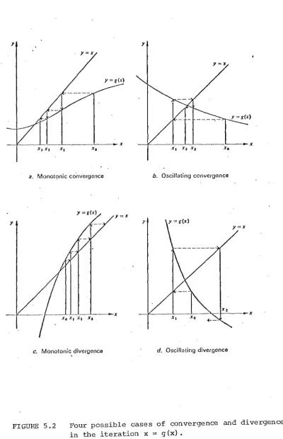
5.2 Four possible cases of convergence
and divergence
5.3 Solution of y'
=
x+y, y(O)=
0, usingEuler's method and 4-step Adams-Bashford
method
5.4 Cubic spline approximation on
a set of (x,y) pairs
57
65
FIGURE
C1
C2
First output from the teaching session
Second output from the teaching session
C3 Third and final output from the teaching session
D1
D2
Output from the first teaching session
Output from the second teaching session
D3.1 First output from the third teaching session
D3.2 Second output from ·the third teaching session
Page
118
119
120
131
14 '1
156
TABLE
I
II
III
LIST OF TABLES
Ordinary Differential Equations
Non-linear Equations
Interpolation and Approximation
Page
75
76
ABSTRACT
NATEP is an interactive computer system with a graphical display. It uses a simple dialogue written in
'STAF' Author Language for ·the user-system communication. A wide selection of numerical algorithms have been
implemented with the facility to enter own functions and data. Plotting routines have been written to provide the graphical output.
In this thesis, .recent and current interactive computer systems used as an aid to solving Numerical Analysis problems are reviewed, and the requiremen·ts for
CHAPTER ONE
IN'l1RODUCTION
In the study of science and engineering the physical laws governing a particular real life process
are represented or modelled by mathematicai equations. Similar methods are being used within other areas such as medicine, economics, and social science. These equations may be algebraic equations, differential equations or integral equations for which ·there are usually two alternative me·thods available for their solution.
One approach is to proceed by the methods of
conventional mathematical analysis in order to obtain the solution in ·the form of a formula or a set of formulae. Inspec·tion of this mathematical solution may then yield qualitative results of interest. If quan·titative results are required, they may be obtained by substituting
numerical values in these formulae.
The alternative method is to solve the equa·tions
Indeed, often, numerical solutions can lead to an understanding of the nature of ·the solution of a problem, sometimes leading to the obtaining of a mathematical
solution. For example, from the numerical results i t may be observed that one quantity varies exponentially wi-th respect to some other quantity, that some variable has only a second-order effect on the result, and so for-th.
Numerical analysis is now, in many situations, the preferred method for the solution of equations
representing a mathematical model. Some·times, even when analytical solutions exist, i t may be preferable to go back ·to the original equations and solve these equations
numerically.
With the advent of digital computers, numerical analysis has become a major part of ma·thematics taught at colleges and universities leading to an expansion of tmdergraduate courses. The course in numerical analysis involves a study of the various numerical techniques available for the solution of a problem and as the
course progresses i t becomes important to have practical assignments completed in order ·to demonstrate a proper understanding of the underlying concepts. A few of the numerical algorithms studied in class can be tested and evaluated by using simple arithmetic but as the problem becomes involved a desk calculator may be used, and in certain cases i t is necessary to use a computer.
analysis. The specific syntax of the individual progranuning language has to be learnt, and as most of the student
programs are often run in a batch·~processing mode, the results may not be known for some hours or even days after submission of the input. Output from the computer is
generally in the form of a list of numbers, and such a presentation usually needs a careful study ·to determine the behaviour of the solution using a particular numerical algorithm.
To remove these extraneous impositions and allow students to concentrate on understanding the ideas of numerical analysis, teachers of numerical analysis
(Corliss 1976; Sumner 1974; Broughton 1976) have realised the need for the following:
1. ( i) Inunediate feedback of resul·ts to the s·tudents. (ii) Inunedia·te feedback of the effec·ts on the
results of varying any parameters in a problem or ·trying a different numerical method.
2. Some form of graphical display of these numerical results.
The basic requirements to sa·tisfy the above needs are: a. A readily accessible computer with ·sufficient s·torage
space to store data and results before being plo·tted. b. An interactive terminal to act as an input/output
device.
c. A graphic device for displaying the results.
An evaluation of an interactive display system for teaching Numerical Analysis carried out at the Universi·ty of North Carolina (Oliver and Brooks 1969) indicated that such a system was a valuable and powerful aid in teaching selected topics in numerical analysis. Also, Sumner (1974) summarizes the opinions of his colleagues at the University of Reading, England, on the use of an on-line facility in teaching numerical analysis. The general conclusion was similar to ·that obtained from the evaluation at North Carolina.
From the above discussion i t is felt that an interactive computer system with a graphical display is of considerable value as an aid to the teaching of
numerical analysis. Such a system has been developed at the University of Canterbury, New Zealand, and is called NATEP (Nwnerical ~nalysis Teaching Package) • It operates
through a simple DECwriter terminal linked ·to the
University's Burroughs B6700 computer with the graphic output produced on a Hewlett-Packard X--Y Plotter.
NATEP provides the following facilities as a teaching aid:
(i) Interaction between the student and the computer through a simple dialogue which may include textual and numerical input from the student, and questions, messages and results to the student. The dialogue is written using the STAF (Science Teachers'
Authoring Facility) Author Language (Peterson 1976). (ii) Numerical algorit.hms in three topics of numerical
of problems. Three areas of numerical analysis currently included in NATEP are the solution of ordinary differential equations, the solution of non-linear equations, and interpolation and
approximation.
(iii) A set of plotting routines to display the numerical results graphically on the plotter. The output can be a series of curves superimposed on graph paper. (iv) The facility for the student to define his own
functions and input data such as initial parameters for a problem or coefficients defining a particular numerical method.
(v) An immediate feedback of the effects on the results of varying any parameters in a problem or trying a different numerical me·thod ·to solve the same problem.
'rhis thesis describes the work carried out in the development of NATEP. Chapter Two surveys and analyses interactive computer systems for numerical analysis
developed in ·the pas·t to illustrate their common fea·tures and their strengths and weaknesses.
Chapter Three describes ·the requirements of a user of an interactive computer system designed as an aid to
teaching Numerical Analysis. It also justifies the approach taken in the development of NATEP.
In Chapter Four the developmen·t of NATEP is described. This includes the interactive language used for the student-system communication, the NUMERALS module which includes the numerical algorithms and the .Plotting routines 1 and the
student and the NUMERALS module.
Chapter Five describes the three topics of
Numerical Analysis implemented in NATEP with a detailed description of the methods and the algori·thms, and a general graphical display of the results.
CHAPTER TWO
SURVEY OF INTERACTIVE COMPUTER SYSTEMS FOR NUMERICAL ANALYSIS
2.0 INTRODUCTION
In Chapter One the need for a computer aid in the teaching of numerical analysis at Universities and Colleges was discussed. This chapter surveys and analyzes systems that have been developed in ·this area in order to illustra·te their common features and their strengths and weaknesses. The systems chosen for this purpose are:
1. The Culler-Fried System (Ruyle, Brackett and Kaplow 1967; Smith 1970b; Ruyle 1968).
2. The AMTRAN System (Ruyle, Brackett. and Kaplow 1967; Smith 1970b~ Wood, Reinfelds, Seitz and Clem 1966J Wood, Seitz and Ely 1968).
3. NAPSS (Symes and Roman 1968; Roman and Symes 1968; Smith ·J970b; Rice 1968; Symes 1970; Rice 1973) .. l~. PEG System (Smith 1970b; Smith 1970a).
5. Kent On-line System (Sumner 1974).
6. Computer Graphics Assisted Numerical Analysis Instruction (CAI) (Corliss 1976).
AMTRAN is used mainly as a service to research scientists and engineers. Culler-Fried and NAPSS also provide such service, but in addition, are used for teaching purposes. PEG system is an example of a special purpose system which is limited to a specific problem area. The other two
systems ~- Kent On-line and CAI are used only in the ·teaching of numerical analysis at Universities and Colleges.
In sections 2. 1 to 2. 6, each of the six systems will be described and in section 2. 7 their s·trengths and weaknesses will be discussed.
2. 1 THE CUI,LER-FRIED SYSTEM
The Culler-Fried Sysi:em is one name for two
physically separate but direct descendants of ·the system originally developed by Culler and Fried (Ruyle, Brackett and Kaplow 1967) a·t Thompson Ramo Wooldridge, California. Since then the On·-line Computer System (OLC) has been
implemented at the University of California at Santa Barbara which operates on the same computer as the original. I t is used for research and teaching on thf:?! Santa Barbara Campus and is available at Harvard University by means of remote ·terminals. The OI,C version has been implemented on a small stand alone system, wi·th drums and magnetic tapes available
for the storage of data and programs.
exponential, and forward difference. The keys for numbers are grouped in the lower half of the keyboard.
An associated storage oscilloscope provides the ou·tput of the results.
The Culler-Fried sys·tem functions roughly like a de-sk calculator, in that the user initiates all calculation by pushing but·tons, with results being displayed numerically and/or graphically on the oscilloscope. A user~defined operator called a CONSOLE program is available whereby the user enters a sequence of system operators and attaches ·the sequence to a button on the keyboard so that subsequent pushes of the button will execute the sequence. These
console programs may call other console programs to a considerable nesting depth introducing a corresponding "pyramiding" of execution times (Ruyle et aZ. 1967).
A partial list of operators (Smith 1970b) provided is:
+ I •• I SIN I STORE I LOAD I DISPLAY •
The source language in the system is such that a fol."'l1Ula has to be expressed in an inside-out fashion where i t has to be entered algorithmically rather than as a normal rna·thema tical expression (Ruyle et aZ. '196 7) . For example,
the formula SIN (x2
+
1) is expressed as: Take XSQUARE X ADD ONE
Take SINE of ·the result.
from the point of correction. Error messages have been entirely omit·ted from the system because of the lack of memory available to do error checking on input.
An example of a ·typical input to the Culler-Fried system is
LOAD X SIN STORE S DISPLAY S
The above sequence of operators will display the SINE of X as a function of X on the CRT where X has been stored in one of the two working registers available.
2.2 THE AMTRAN SYSTEM
The AMTRAN (Automatic Mathematical Translation) System was developed at the NASA Marshall Space Flight Center in Huntsville, Alabama (Smith 1970b). It is a
time-sharing remote-terminal computer system in·tended to permit users ·to solve problems using the standard
mathematical notations and its main use is in the field of research by sci en tis ts and engineers.
Implemented on a small stand alone system1 AMTRAN
has its main application through in·terac·ti ve ·terminals. These terminals consist of a large keyboard (Wood,
Reinfelds, Seitz and Clem 1966), two 5-inch storage oscilloscopes for graphical and alphanumeric display, and a typewriter to provide a permanen·t record.
'rhe AMTRAN system provides for automatic array arithmetic, automatic dimensioning of arrays, automatic assignmen·t of working storage, implied multiplication, and input and output in standard mathematical notation. Adaptive Numerical Analy·tical Problem Solving Routines
(Wood, Seitz and Ely 1968) are available for use. Typical routines are
-REPRESENT - Numerically represents mathematical formulae, selecting near optimum step size assuming a cubic polynomial fit. Automatically detects singularities and discontinuities.
DERIV Calculates the numerical derivative using a cubic fit.
Input for a mathematical formula such as SIN(X2 + 1) is in an infix form (Ruyle, Bracket·t and Kaplow 1967), i.e. the formula is expressed in the customary fashion as the sine of the sum o:f one and the square of X. Program editing in AMTRAN permits whole command lines to be inserted in a program or existing command lines to be replaced.
An example of a typical input where the user has ·to know the correct sequence of operators which is obtained
from the guide on ·the use of the Adaptive routines is:
REPRESENT 7' 1, 2 y
=
rrAN X2.3 NAPSS
The NAPSS (Numerical Analysis Problem Solving System), developed at Purdue University, West Lafayette, Indiana, is implemented on a CDC 6500 (Rice 1973) and runs in a time-sharing environment at on-line remote consoles which include graphics capabilities. NAPSS programs which can also be executed as batch jobs are used for teaching as well as for solving problems in numerical analysis (Smith
1970b).
Five general techniques have been utilized to assist the user in stating and solving a problem (Symes 1970):
1. The source language used to present a problem to the computer is similar to normal mathematical notation. 2. Statements used for dimensioning arrays and declaring
variables are removed from the source language as ·these tasks are done by the system.
3. NAPSS penni ts the direct use of quanti ties other than scalars. These include numeric arrays, symbolic
expressions and functions.
4. The use of polyalgorithms reduces the amount of problem analysis needed before the problem is presented to the system. A polyalgorithm is formed by the synthesis of a group of numerical methods and a logical structure into an integrated procedure for solving a specific ·type of mathematical problem (Smith 1970b).
and the system is able to request information and indicate errors when they arise.
Typical polyalgorithms available in NAPSS (Smith 1970b; Rice 1968) are:
Integration Interpolation
Solution of non-linear systems
To solve commonly occurring problems the user need only supply to the system a description of the problem to be solved and the variables to be found; a knowledge of the numerical analysis involved is not required (Symes and Roman 1968). rrhe. method is selec·ted by the system with the aid of the polyalgorithms which attempt to solve the problem au-tomatically and request additional informa·tion as needed and monitor the accuracy of the results.
2. 4 PEG SYSTEM
PEG is an example of a special purpose sys·tem, in this case for on-line solution of least squares data-fitting problems developed at the Stanford Linear
Accelerator Center, S·tanford University, California.
I t has been implemented on an IBM 360/91 Computer with an IBM 2250-II display unit (CRT with light pen and keyboard) .
All the user actions are either by lightpen selection of the op·tions displayed on the CRT or the keyboard entry of
numbers for flpecifying degrees of fit and in some cases initial values for parameters. The list of options available for on-line selection are accomplished by
user selection, ·thus avoiding the entry of invalid requests requiring diagnostics.
The PEG system allows user selection of:
1. Choice of Function- this display allows the selection of a fitting function and the currently available
choices are: orthogonal polynomials, spline functions, and user defined functions.
2. Choice of Input Mode - the methods of entering data in·to the system are: data cards, keyboard entries, and data from previous fit.
3. Choice of Display Mode - after the fit has been calculatedthis display allows for a choice from a list of display modes which will show graphically and numerically the results of the fit. These displays will graph the data wi·th the fitting func·tion
superimposed, show a table of residuals, graph ·the residuals, or show the numerical values of the parameters of the fit·ting function.
In addi"ti.on to the above, the system allows specification of the degree of interpolation, initial
guesses for non··· linear problems, and choice of minimization problems. With all these facilities available, PEG is
oriented toward the non-programmer.
2.5 KENT ON-LINE SYSTEM (KOS)
programs, collectively known as MATHLAB.
Input to KOS consists of commands and data via
teletype consoles or some other source such as a disk file. Output is printed on the teletype and consis·ts of messages
and results.
Some of the MATHLAB programs are library algorithms designed to do a specific task such as S'rURMC which
calculates the eigenvalues of a symmetric ma·trix and is intended to provide a service to chemistry students working on molecular orbitals rather than to teach the Sturm
sequence method as such. Most of the programs, however, ask for a posi·tive contribution from the user, who is then in an active learning situa·tion.
A few of the subjects implemented in KOS are: 1. Interpolation
2. Solution of non-linear algebraic equations 3. Solution of Ordinary Differential Equations 4. Solution of linear equa·tions
5. Calculation of the eigenvalues of a matrix.
2. 6 COMPU'rER GRAPHICS ASSISTED NUHERICAL ANALYSIS INSTRUCTION (CAI)
The CAI system was developed at the University of Nebraska, Lincoln, and consists of a computer assisted instruction package for numerical analysis in a first year course (Corliss 1976). It is implemented on an Interdata Model 70 mini--computer, and peripherals to the sys·tem include a teletype console and a Tektronix 4002A storage tube.
Topics in numerical analysis included in the package are:
1. Root- finding
2. Fixed-point i tera·tion 3. Polynomial interpolation
4. Numerical differentiation and numerical integration. The user communicates vvi th the CAI system ·through a cross hair cursor, or through a keyboard, and the system is used to assist numerical analysis ins·truc·tion in two ways: 1. An instructor may use the package for a demonstration
which enables him to in·troduce a new algorithm to ·the class by showing how the algorithm works on several different problems.
2. The studen·ts use i t to explore at their own pace the action of the algorithms being studied in class.
2.7 DISCUSSION
For any interactive sys·tem, the method of inpu·t is quite important. Use of a special keyboard as in Culler-Fried and AHTRAN; will facilitate ease of operation,
once the user is familiar with its layout, but the extra cost of developing and interfacing such equipment generally makes i t unavailable for all but ·the largest users of such systems. Although this type of keyboard can· assist user responses ·they may be harder t:o learn. On the other hand, general keyboard facilities, as in NAPSS, are convenient to use but require a more .detailed inpu·t. The use of a light-pen on a graphics display to.select data from a 'menu' of choices, as in PEG, is another alternative form of input. However, such a graphic system is expensive to buy and requires a greater software support.
Another important consideration for any interac·tive system is the source language used.· The Culler-Fried system requires a formula to be expressed in an 'inside-out'
fashion. Any system whose source language does not resenmle normal mathematical language would be inconvenient to use. AMTRAN, NAPSS, KOS and the CAI systems are suitable in that their source language resembles closely the standard
mathematical form and does not put any undue burden on the user in expressing a formula or a problem.
The facility for editing and B1e provision of
whole conuuand lines to be replaced or inserted in a program. Of all the systems discussed, NAPSS is best equipped in terms of the editing facility and the display· of error messages.
An interactive system with graphics capability provides the facility to display graphs similar to ·those which migh·t be drawn by hand on the blackboard or on graph paper. The five systems - Culler-Fried, AMTRAN, NAPSS, PEG and CAI - provide this capability with the KOS system being restricted to output on the teletype only.
The most significant feature of an interactive system is the usefulness of such a system to the user. NAPSS with its source language similar to the standard ma·thematical nota·tion, with its editing facility, graphic capability and
the use of polyalgorithms is most convenient for teaching purposes. It has also found use as a service to research scientis-ts and engineers as have the Culler-Fried and AMTRAN. A special purpose system, such as PEG, is useful in teaching but limits the teaching to only one topic or area. The KOS system has been found by the teaching staff at the University of Reading, England, to be a useful aid in ·teaching
2 • 8 S UMl.'1ARY
From the above survey of interactive computer systems for numerical analysis, i t can be noted that there is no completely suitable system available for teaching purposes.
NAPSS has most of the facilities desired in a teaching
system, but its size and associa·ted hardware and software make it unavailable for all but the largest users of such
CHAPTER THREE
REQUIREMENTS OF AN INTERACTIVE COBPUTER SYSTEM FOR TEACHING NUHERICAL ANALYSIS
3.0 INTRODUCTION
Chapter Three discusses the requirements of a system designed to assist in the teaching of numerical analysis. This is followed by a justification of the approach taken in ·the design of such a system, and the chapter concludes with a brief description of the sys·tem developed a·t the University of Canterbury.
3.1 EVALUATION OF AN INTERACTIVE DISPLAY SYSTEM
An evaluation of an interactive display system for teaching numerical analysis was carried out by the
Department of Computer Science and Information Science at University of North Carolina (Oliver and Brooks 1969). A brief non-·credi t course in elementary numerical analysis was offered to b~10 groups; one group being taught with the aid of an on-line graphic system, the other being taught using the conventional teaching methods. The topics of numerical analysis included in the. course were:
1. Numerical solution of Ordinary Differential Equations. 2. Polynomial Approximation and Interpola·tion.
The following conclusions were made from the results of the experiment:
1. Class participation was much grea·ter in the first group (the one using the on-line system) and the students in this group were eager to pursue topics which were not directly covered in the lectures. Also, the performance of ·the students in this group was bet·ter in the
examinations than those from the second group using conventional teaching methods.
2. Immediate response to questions stimulated s·tudent interest in the subject and s·tudent retention of the subject matter was 'improved.
3. The interactive graphics system performed better than visual facilities generally used, as i t provided a
flexibility not available through slides or film strips. Finally the results indicated ·that the interactive display system was a valuable and powerful aid in teaching selected topics in numerical analysis.
3. 2 USER REQUIRENENTS
In order to fulfil the needs of a user, ·the basic requirements of an .interactive computer sys·tem wi tll graphic display for teaching numerical analysis are considered to be:
1. A set of numerical algorithms for different topics in numerical analysis.
2. A set of routines to handle user-defined functions and data.
numerical results obtained from the various numerical methods.
4. An effective user-system communication.
3.3 JUSTIFICATION
3.3.1 Numerical methods
The choice of different subj ec·ts in numerical analysis and ·the various methods within these subjects are based on the fact that one is not seeking the 'best' algorithms for solving problems but for educational purposes i t should be possible to be able ·to .use many different algorithms in order to compare results. The reasons for this are as follows.
Besides being concerned with numbers, errors and algorithms (Wilkinson 1963), numerical analysis also
involves the problems of ins·tabili ty and ill-conditioning. Instability_ describes the phenomenon where t.he round-off errors instead of compensating each other to a large extent grow exponentially and affect ·the final resul·t grea·tly. Ill-conditioned problems are those where small changes in initial data may produce a large change in t.he final resul·t.
For example, the general 2-step explicit linear multistep formula for the solution of the initial value problem,
y' (x)
=
f(x,y(x)), y (x )0 == y ' 0
is Yn+1
=
a1yn + a2yn-1 + h(Sifn + f32fn-1)' n=
1 ,2,3, ••• where y is a numerical approximation to y(x ) andn n
fn ~ f(xn,yn). The coefficients a
S
1
=
2 ands
2=
0, then the resulting formula is Milnes second order formula,=
y n-1 + 2hf ' n n==1,2,3, ...•.If this formula is applied to the ini·tial value problem
y'(x)
=
-2y(x)+
1, y(O)=
1,then a plot of the numerical solution for h
=
0.125 andN
=
32 and a plot of the true solution y (x)=
!e -2x+
0. 5 (Figure 3. 1) shows how ·the numerical solution oscillates about the true solution with the error growing in an exponential manner. Thus ·the theoretical result that Milnes method is unstable is demonstrated.In ·the approximation of data or functions, the basic approximation used is a polynomial. One \vay of writing a polynomial p (x) of degree n, passing ·through (n
+
1) data points (x, ,f(x.)), i=
0(1)n, is in terms of the Lagrangel l
polynomials L. (x). That is,
J
p (x)
L. (x) J
=
=
n
E
j=O
n
IT i==O
i~j
f ( x . )
r .. (
x)J J
(x - xi)
(x, -x.) J l
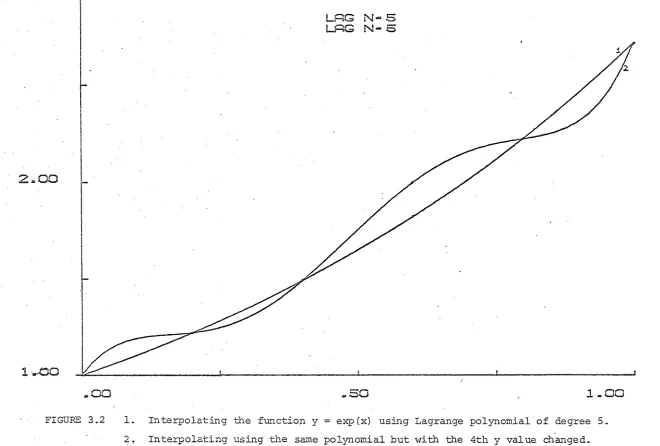
Because of the oscillatory nature of polynomials,
especially as ·the degree increases, interpola·tory
polynomials such as the above can be very sensitive to
~50
.00
12
t
I
I
\
1
I
.00 2 . 0 0 4 . 0 0
'FIGURE 3.1 Use of Milne's Second Order Formula (2) y
1 = y 1 + 2hf , n = 1,2, ...
n+ n- n
I
I
to ~olve.y' (x) .= -2y(x) + 1, y(o) ·= 1 with the true solution y(x) = ~e-2x+! (1).
N
-.:.'lritten in the conventional form
p (x)
=
'rhis is the problem of ill-· conditioning. Ill-conditioning can be illustra·ted by first plotting the polynomial for a given da·ta and then replotting the polynomial for the same da·ta with say, one function value changed as shown in
Figure 3.2. Again the relevance of the theoretical results can be appreciated by seeing the effect in prac·tice.
To provide the various numerical me·thods in different topics of numerical analysis, two of the alternatives
available are:
(i) to use program packages, and
(ii) to develope one's own set of algorithms.
Program packages, such as Burroughs Numerals, will normally contain some of the best methods available for solving problems numerically. The various problems of numerical analysis can be solved using this package by passing the necessary parameters to the methods. However,
this may be of limited value in the educat.:ional field where i t is necessary to compare numerical results from different numerical methods to demons·trat.e the st.rengths and
weaknesses of these algori ·thms and to illustrate some of the problems of numerical analysis such as instability and ill-conditioning.
2 .. 00
1-...CO
.. oo
FIGURE 3.2 1. Interpolating the fu.11ction y
LRG N-S LAG N-S
.. so
1 .. 00exp(x) using Lagrange polynomial of degree 5. 2, Interpolating using the same polynomial but with the 4th y value changed.
N
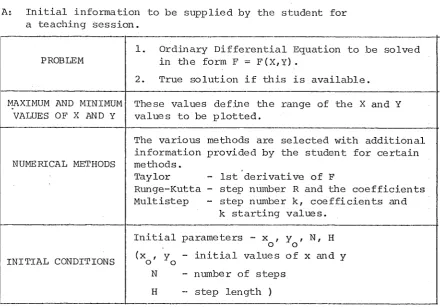
[image:36.842.108.768.59.505.2]problems of numerical analysis. The facilities to enter one's own coefficients to define some of the numerical methods, for example, Multistep me·thods for the solution of ordinary differential equations, can be included in these algorithms.
There are two possibilities for computer processing of these numerical algorithms - comple·te interpretive
execution of each of the algorithms or the use of
precompiled algorithms. Due to the fact that numerical analysis problems rely heavily on iterative processes, a high percen·tage of the statements in the algorithms will be expected to be execu·ted more than once. Considering the differences in time taken in compila·tion and interpreta·tion, ·the use of precompiled algorithms which can be directly
used repeatedly is more preferable than the interpre·tive execution of the algorithms. However, this approach does no·t restrict ·the user selection of functions and data.
3. 3. 2 User-defined functions and data
To solve and study a wide range of problems in
numerical analysis i t is essential to have the facility to be able to enter one's own functions or polynomials, initial parameters and coefficients. The functions and data should be able to be changed readily and ·the various numerical
algorithms being studied can be tested in full. Indeed, the student should be able to construct his .own methods so that the effects of not satisfying theoretical
or Runge-I<utta formulae for the solution of an ordinary differential equation, by supplying the number of steps and the corresponding coefficien·ts.
During a teaching session the student would be required to input functions and data of his own choice. These functions and data can be processed by the computer in one of two ways - compilation of functions and data or interpretive execution of the input.
With the first approach, ·the func·tions entered would be compiled separately and combined with the object
code for the algorithm being used. While the ultimate execution speed is significantly faster, the major
disadvantage associated with this method of operating is the inherent delay in response caused by the extra steps of compiling and combining (binding) ·the studen·t' s function. During this time, no execution of ·the main program takes place and the delay can be most unsatisfactory for the user.
The second approach is to execute the fw1ctions and data interpretively as they are entered by the student. Although the major disadvantage of interpretive execution is the time consideration, i.e. its operation is at a slower speed than a compiled program, the response to the student is usually satisfactory.
3.3.3 Graphical display of results.
When dealing with problems in numerical analysis most of the ouptut is in the form of a list of numbers,
and such a presentation usually needs a careful study to observe the behaviour of various numerical algorithms. In some simple cases, i ·t may be possible to visualize how an algorithm works by looking at a table of numbers but this may not be possible always.
The other alternative is to plot these numbers on graph paper and study the graphical results for the various numerical methods but this approach may be
·time-consuming and laborious. These impositions suggest computer production of graphical results so that the analysis of algorithms is made simpler and faster.
Graphical representat.ion of numerical results illustrate the actions of the algorithm and the effects of changes in problem parameters on the solution
and demonstrate the properties of instability and ill-conditioning in some of the numerical methods.
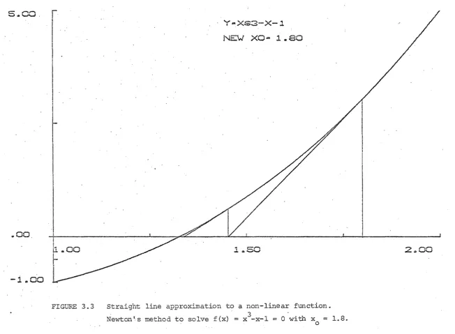
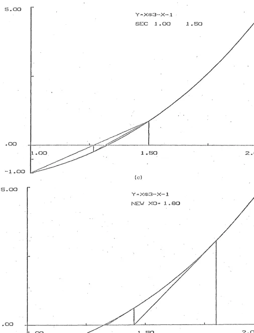
'l'h.is form of the presentation of results also highligh·l:s the fundamental principle of numerical analysis that occurs ·throughout the cons·truction of methods for the solution of problems. For example, in ·the iterative solution of
non-linear algebraic equa·tions, straight line approximation. to the non-linear function is used in some of the standard methods such as Bisection, Regula Falsi and Newtons's
.. oo.
-i ..
OO
NE'v..' XO ... 1.80
I .
f
I
I
'1 .. 50
FIGURE 3.3 Straight line approxLmation to a non-linear function.
Newton's method to solve f (x)
=
x3 -x-1=
0 with x=
l . 8.0
2 .. 00
w
[image:40.844.108.760.52.530.2]tangent to the function curve. Such representation of these methods should lead one ·to consider approximation other than linear approximation as a natural ex·tension of this concept.
3.3.4 User-system con~uni~ation
In ·the design of an interactive system for teaching purposes, a very important considera·tion is the appearance of the system to the user (the man-machine interface). It should be designed so that any user can understand
what is happening and what is expected of him at each step. This requires an effec·tive user-system communication,
and some of the alternative methods of communication are as follows:
(i} Specifying parameters to a package
Using a package such as Burroughs Numerals requires the user to -specify the problem ·to be solved, enter the name of the numerical me·thod to be used, and
supply the necessary parameters. 1'he package in turn produces the numerical resul·ts. This approach does not allow one to chang·e parameters or to choose different methods to compare resul·ts, both of which are essential for teaching purposes. It limits the options available to the user after a specific
problem is solved.
( ii) ;Light-pen s elec·tion of options
specify that optiori, thereby eliminating the need for entry of alphabetic commands. Although this form of communica·tion is faster than keyboard entry of commands and is generally easier to use,
graphics systems are usually expensive and require considerable software support.
(iii) Keyboard entry of numbers
For this form of communication the options,
numbered sequen·tially, are presented at a teletype or typewriter terminal. These options could
include the names of the topics of numerical analysis and the various numerical methods implemented. 'l'he user selects his option by typing in the number corresponding to his choice. Numeric data and functions can likewise be entered through ·the keyboard.
Altho'l.1gh this me·thod of communication is
straightforward i·t has limitations. The method is restrictive as i·t offers a fixed number of choices and i t does not allow the user to deviate from the available menu.
(iv) A simple dialogue
Another alternative for the communication between the user and the system is a simple dialogue
inputs from the user to avoid introducing tmnecessary typing errors. With a simple dialogue the user will have flexibility in the choice of input and any
sensible input could be accepted. Also there cru1 be a facility whereby the student response is recorded continuously, and the response matching scheme can be upda·ted to allow for a wide range of responses from the s·tudent. However, this form of communica·tion, which would require cons·tan t use of the keyboard, may be inconvenient in that the user may have initial difficulty because of lack of familiarity with b~e keyboard. Subse·quently with frequen·t use of the system, the keyboard should become familiar and more convenient to use.
Of the four alternatives discussed above, each of them has its meri·ts and limitations. Although a utili·ty package such as Burroughs Numerals is convenient in that i t is readily available, specifying parameters to such a package is unsuitable for teaching purposes. The use of a ligh·t-pen device which is usually complemen·ted with a keyboard would be ideal for the user-system communication, but i t is expensive to acquire nnd may not be readily
available. Keyboard entry of numbers for connnunication is easy ·to use and may be cheaper to implement, but i t is not a convenient form of communication. Using a suitable interactive language, a simple dialogue for ·the
light-pen device.
Considering the availability, simplicity, usefulness and ·the cos·t of the alternatives for the user-system
communication the·choice of a simple dialogue may be the mo s·t appropriate.
3.4 A COMPUTER AID FOR TEACHING NUMERICAL ANALYSIS
To satisfy student needs as discussed in the above sections, NATEP, an aid to teaching numerical analysis was developed. It consists of ·two major parts:
1. A NUMERALS module 2. A CONVERSATION module
The NUMERALS module fulfils the student requirements as discussed in sections 3.3.1, 3.3.2 and 3.3.3. It
provides the studen·t with a wide selection of numerical algorithms to solve problems, and the plo·tting routines to dra-vr graphs of the numerical results. It handles user-defined functions and data to be used in ·the numerical computations.
CHAPTER FOUR
DEVELOPMENT OF NATEP
4.0 INTRODUCTION
Chapter Four describes the development of NATEP. It discusses the interactive language used for the dialogue between the student and the sys·tem, the implementation of the language, the CONVERSATION module, the NUMERALS module and the plotter.
4.1 INTERACTIVE LANGUAGE
4.1.1 The 'Staf' Author Language
A sys·tem providing Compu·ter Assisted Learning· in Chemistry has been developed in the Chemistry Department at the University of Canterbury ('1977). This implementation is based on CALCHEM (Computer Assisted Learning in
Chemistry), a project of the United Kingdom National Development Programme in Computer Assisted Learning
(Peterson 19 7 6) . The proj ec·t uses. STAF ·(Science Teachers' Authoring Facili·ty) Author Language as the in·teractive language to provide the dialogue between the student and
i:he system.
As the STAF Author Language satisfies the basic requirements of an interactive language to be used in a computer aid to the teaching 'of Numerical Analysis
University of Canterbury computer, i t was decided to make full use of this facility rather than to design and
implement a new language. The S'rAF Author Language provides the following capabilities:
1. Output of messages and questions to the student. 2 ._ Recognition of textual and numerical input from
the student.
3. Control of the dialogue between the s·tudent and the computer system using a 11 branching-tree .. structure.
4. Interface into external routines which handle numerical computation.
5. Recording of the dialogue sequence ·to provide feedback to the teacher on the suitability of the conrrnunication.
4.
·t.
2 Description of 'STAF' teaching prog_raiTll!le NATEP uses the Burroughs ALGOL version of the S'l'AF Author Language (University of Can·terbury 1977) whose syntax is described in Appendix A. A file of text writ·ten in ·this language is referred to as a STAF teaching programme.The teaching progranrrne is divided into a ntrr®er of nodes forming the basis of a branching tree structure. These nodes must con·t:ain:
1. A unique iden·tifier which assigns a name ·to the node. 2. Routing ins·tructions which route ·the students i.:o other
nodes of the tree structure as a result of their responses.
They may also contain:
2. Hatching schemes to allow for the interpretation of the student responses.
3. Calls to external subroutines which may include numerical procedures and plotting routines.
4.2 IMPLEMENTATION OF STAF AUTHOR LANGUAGE
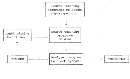
The implementation of the STAF Author Language for the B6700 computer required a program called Analyser which was developed by B.L. Harper of the Chemistry
Department of the University of Canterbury. Its function is to validate the STAF teaching programme which may be edited using the standa.rd CANDE (_g_ommand AND :§_dit)
facilities of the Burroughs B6700 computer (Drawneek 1975) and to produce a file called the Teachfile which consists of a table of nodes forming ·the structure of ·the student~
system dialogue. Figure 4. 1 illustrates ·the development of ·the teaching programme and the •reachfile.
CANDE editing facilities
I
TEAC~ER
l
+Source teaching programme on cards,
papertape, etc.
- - - - +
!
Source teaching
I
programme on disk
l
_ _ _ _
~alyser
programL~o check syntax - - - - +
r
'l'EACHFILE [image:47.598.67.539.55.797.2] [image:47.598.85.519.511.775.2]4.
2. 1 Devel_sement of the teachir.!SLProgrammeIn the development of a teaching programme the preliminary steps are:
1. A summary by the teacher of the topics of numerical analysis and ·the numerical algorithms within these topics to be made available to the student.
2. Establishment of a tree structure consisting of a sequence of questions, answers and messages to assist in teaching.
3. Concise formulation, in plain English, of the sequence of questions described in (2) and the various acceptable ·responses from the student.
The teaching programme is then coded according to the STAF Author Language syntax, and can be punched on to cards and loaded on to a disk file. Alterna·tively
the ·teacher could create the file directly through the CAL\fDE f aci l i ty.
4. 2. 2 Crea·ting the Teach file_
'rhe Analyser program checks the syn·tax of the teaching progran®e and generates the Teachfile. Syntax errors or other STAF language violations will be identified and corrections may be made by editing the teaching
programme file through the CANDE facility or crea·ting a new corrected teaching programme. When all the errors have been removed, the Teachfile is generated. Once created, the Teachfile does not require to be changed unless some modifications such as, for example, addition of further
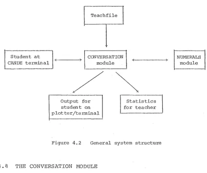
NATEP consists of two main parts - the CONVERSA'riON module and the NUMERALS module. The general s·tructure of NATEP is illustr~ted in Figure 4.2.
Student at .
J
+ - - - - + CAI.\IDE termmalTeachfile
CONVERSATION
module - f - - - >
I
NUMERA~S
modulek
Output for student on otter/terminall s t a t i s t i : - J
I
for teacherI
Figure 4.2 General system structure
1-J.. L!. THE CONVERSATION MODULE
The CONVERSATION module as implemen·ted in NATEP interpre·ts the student responses and provides an interface be·tween the Teachfile and the NUMERALS module which contains the numerical algorithms and the plotting routines. It
[image:49.597.92.518.215.571.2]or calls to the numerical algori·thms and ·the plo·tting
routines.
4.4.1 Besponse matchin~
When designing the teaching programme, ·the teacher lists a series of anticipated respcinses to a particular question at a node where a student response is expected. The student response at that node is then compared with the anticipated responses and the appropriate r·outing is
implemented. Following the last anticipated response there is a 'direct routing' which is followed if no successful match is made.
In determining what anticipated responses to include for a question or request, the following steps have been found to be generally useful.
1. For a question whose answer is either in affirmative or in the negative, commonly occurring responses like yes or no, yap or na, or even the first letters of the words yes and no, may be included.
2. When the inpu·t is to be ·the name of a numerical topic or a numerical method or the ·type of a problem,
commonly used names in text books and lectures may be used. Here the first one or two or three letters of the name as necessary should be sufficient if the choice does no·t lead to confusion in names.
sufficient for tl1e first option, and just the name of another numerical method should be enough for the second option •.
A statistics file (called SAVEFILE) is generated by the CONVERSATION module during each of the student sessions. This file con·tains the names of the nodes visited in the course of a dialogue and the corresponding student responses at each such node. The statistics thus collected may help the teacher in determining which of ·the student responses are conm1on and must appear in ·the list of anticipa·ted responses, and if any extra information is to be provided to the student to assist him to respond to a particular question.
4.4.2 Calls to external routines
External routines which are invoked by the CONVERSATION module include the numerical algorithms, the plotting routines, and routines which handle user-defined function and input of data such as initial
parameters, or coefficien·ts defining a particular numerical method. This is accomplished by using the facility of CF commands of the STAF Author Language (Appendix A). When such a call is encountered at a node in the Teachfile no student response is expected at that node, but a call to an external routine is to be made. From the CF command in the Teachfile, the CONVERSATION module iden·tifies the
Ll. 5 THE NUMERALS MODULE
4.5. 1 Numerical algorithms
The three topics in Numerical Analysis which have been included in NATEP at the present time are:
1. The solution of Ordinary Differen·tial Equations (first order, initial value p~oblems).
2. The solution of a non-linear algebraic equation. 3. Interpolation and Approximation.
These three topics form a significant part of
undergraduate numerical courses at Universi·ties. Further, the underlying principles of the numerical methods in ·these subjects can be well illustrated by graphical methods. As NATEP is designed so that further subject areas may be
readily included, ·the sys·tem is not restricted to only these three subjects. The numerical algori·thms which have been implemented for the three topics are described
in
Chapter: Five.
Each of ·the numerical methods is implemented as a numerical procedure which can be invoked by the CONVERSATION module. The numerical procedures are independen·t of each other, which facilitates the addition of further numerical methods.
4.5.2 ?lotting routines
maximum and minimum X and Y values are supplied to define the range of the X and Y coordinates. The axes are drawn according to ·these values with a grid marked, and on request these axes can be labelled. Each of the curves plotted may be labelled and a differen-t colour of ink for the plotter pen could be used to differentiate between the curves.
The numerical procedures call these plo·tting routines and pass the computed X and Y values for a problem. These X and Y values are then scaled according to the maximum and minimmn values of X and Y, and plotted.
4.5.3 User-defined functions
To solve an ordinary differen-tial equation or a non-linear algebraic equation the student would need to supply this equation ·to the system in the course of the dialogue. Routines have been included in ·the NUJY:I.ERALS module to handle ·the input of such user-defined equa·tions
or functions whose syntax is described in Appendix B1. On recognising that the system is expecting a function from the s·tudent these routines are called.
The func·tion is read and the expression is ·translated into a reverse polish string and stored for later use. Before the translation stage the syntax of the expression for ·the function is checked. Upon detection of a violation of the syntax rules, the system responds with appropriate messages to the student, who is then allowed to re-enter the
expression. Appendix B2 describes the conversion of the expression from the infix form to reverse polish form.
mechanism is used to evaluate the reverse polish form of the expressions. During a numerical computation,
interrupts such as, for example, a negative argument for the SQUARE ROOT intrinsic or EXPONENT OVERFLOW in a
variable, will terminate the function evaluation and ·the s·tudent is returned to a node in the Teachfile from which he can either continue with the options available at that node or terminate the session.
In the present implementation of NATEP, the use of scalar variables penni ts the inclusion of major areas of undergraduate numerical analysis courses taught at
university. The implementation of vectors for the solution of systems of ordinary differen·tial equations is feasible but has not been implemented a·t present.
4.5.4
User supplied dataTypical examples of data which need to be supplied to the system in order to solve a particular numerical problem are:
1. Initial conditions of a problem or starting values for a numerical me·thod.
2. Coefficients defining some of the numerical me·thods, for example 1 Multi-step methods for ·the solution of ordinary differential equa·tions.
3. A set of (X, Y) pairs for in·terpola tion where Y
=
f (X) .4.
Polynomial degree a.nd coefficients for a polynomialin X.
Routines have been written to handle the input of the above data. 'l'here is provision in NATEP whereby ·the
student can use ·the system supplied data instead of providi~g his own, and ·this type of data generally includes ·the
standard coefficients for Runge-Kutta methods and Mul·ti-step methods, and selec·ted sets of (X, Y) pairs which can be used in interpolation.
4.6 THE PLOTTER
The results from the various numerical methods may be displayed on a Hewlett-Packard 7202A XY-Plo·tter which is driven as a slave device ·to a DECwriter terminal which is on-line ·to the University's Burroughs B6700 computer. A detailed description of ·the plotter is given in the
Hewle·tt-Packard Operator's Manual (1971) with a summary of the controls and indicators given on the plotter's pull-out instruction card.
Driven as coordina·te pairs, ·the plot·ter accepts the (X, Y) pairs in the range 0-9999 and draws vectors a·t any angle up to 7. 5 em long only. A line of length grea"cer than this is drawn as a series of shorter lines which does not affect the final display in any way.
As the plotter: does not include any hardware or software capability for the labelling of the axes and ·the curves, software has been designed for this purpose.
CHAPTER FIVE
THE NUMERICAL ALGORITHMS
.AND GRAPHICAL DISPLAY OF RESULTS
5.0 INTRODUCTION
Chapter Five describes the three ·topics of Numerical
Analysis which have been implemented. in NATEP. 'rhey are:
1. The solution of an Ordinary Differential Equation (a
first order, single value problem) (Conte and de Boor
1972; Lambert 1973).
2. The solution of a single non-linear algebraic equation
(Conte and de Boor 1972).
3. In·terpola·tion and Approximation (Conte and de Boor 19 72;
Shampine and Allen 1973).
A de·tailed description of the methods and the
algori·thms used is given and the general graphical display
of the results from each of ·the three topics is described.
The chapter concludes with a reference to typical teaching
sessions with NATEP.
5.1 SOLUTION OF NON-LINEAR EQUATIONS
5.1.0 Introduction
The roots of a non-linear equation f(x)
=
0 cannot in general be expressed in closed fo:r.111.. In order to solvethese non-linear equations it' is usual to employ approximate
one or more initial approximations ·to the root, they produce a sequence x
0, x1, x2, . . . which may converge to the desired root. With certain methods, i t is sufficient
(for convergence) to know an in·terval [a,b] which contains the roo·t. Other methods require a suitable initial approximation to the desired root; in return,
these me·thods converge more quickly. Initial approximations to the roots of an equation f(x)
=
0 can often be obtained by graphing the function f (x) .The iterative methods which have been implemented in NATEP are:
BISECTION REGULA FALSI
MODIFIED REGULA FALSI SECANT
NEWTON
FIXED POINT ITERATION
5. 1. 1 Bisection method
Given an interval [a,b] such that f(a) and f(b) are of opposite signs (i.e. f(a) .f(b) < 0), this interval will contain at least.one root of the equation f(x)
=
0.The s·traight line used to approximate the funct.ion passes ·through the mid-point o:E ·the inte:cval [a, b] . 'I'his method locates the solution by halving the original interval, and generates a SE~quence of intervals of decreasing size containing ·the root, always maint.aining the values of the function a·t the end points to be of opposite sign. Although a root can be always located with this algorithm, the Bisection me·thod converges ·to the solu·tion ra·ther
5.1.1.1 ~lgorj·thm
Given a function f(x) continuous on the interval [a ,b ] and such ·that f(a ) f(b ) < 0 •
0 0 0 0
-For n
=
0,1.,
2, ... , until sa·tisfied, do:Set m
=
(a +b )/2n n
If f (a ) . f (m) < 0 , set a == a , b
=
mn - n+1 n n+1
Otherwise, set an+ 1
=
~~ bn+ 1=
bn .Then f(x) has a root in the interval [an+1' bn+ 1
1 •
5.1.2 Regula Falsi
This method is similar to the Bisection method with ·the exception ·that the secant used to approximate the
function passes through the weighted average of the interval rather than the mid-point. The sign of f(x) is examined at the weighted average to ge·t the next: interval containing the root. Although t.he Regula Falsi produces a point at which the absolute value of f(x) approaches zero faster than does the Bisection me·thod, i·t may fail completely to give a small interval in which a root is known to lie. The root is
approached from one side only such tha·t one end of the interval bracketing the roo·t is the final approximation ·to the root whilst the other is ·the original value of one end of the initial interval.
5.1.2.1 Al_9orithm
Given a function f (x) continuous on the interval [a , b ] and such that f(a )f(b) <0.