Controller design for a bipedal robot with variable stiffness actuators

University of Twente

EEMCS / Electrical Engineering

Robotics and Mechatronics

Controller design for a Bipedal Robot

with Variable Stiffness Actuators

J.G. (Jildert) Ketelaar

MSc Report

Committee: Prof.dr.ir. S. Stramigioli Dr. R. Carloni L.C. Visser, MSc Dr. E.H.F. van Asseldonk

December 2012

ii MSc report - J.G. Ketelaar

iii

Summary

This report describes the modeling and the design and implementation of a control architec-ture for a bipedal walking robot. This robot feaarchitec-tures variable stiffness actuators in the knees which make it possible to adjust the knee stiffness during walking. Previous research showed that using the leg stiffness as a control input, a robust and human-like walking gait can be achieved. The proposed controller tries to keep track of a defined walking pattern and fur-thermore uses the variable knee stiffness as a control input in order to achieve a desired leg stiffness. The controller is validated by both simulation and experimental results which show that a bipedal walking robot can maintain a certain gait by adjusting the leg stiffness.

iv MSc report - J.G. Ketelaar

v

Contents

Summary iii

1 Introduction 1

2 Journal paper 2

3 Conclusion and recommendations 12

3.1 Conclusion . . . 12

3.2 Recommendations . . . 12

A Manual 13

A.1 Quick user guide . . . 13

A.2 Troubleshooting . . . 15

A.3 Software . . . 16

B ICRA paper 19

C Guide rail redesign 25

D 20-sim model 26

E Experiment debug scripts 28

E.1 CLW visualization . . . 28

E.2 Posteriori controller calculations . . . 28

Bibliography 29

vi MSc report - J.G. Ketelaar

1

1 Introduction

Since the emergence of robotics, robots have assisted and took over a lot of human activities, especially in factories. When it comes to mobile robots, these devices are often driven by a set of wheels for this is a proven concept and relatively easy to control. A drawback of wheels is however that they require a certain smoothness of the terrain, for example a staircase or a steep hill is hard to approach for a platform on wheels. Because humans nowadays desire more flexible (assistive) robots on terrains which are not suitable for wheels, more and more research is aimed to understand the human locomotion in order to mimic the mobility of humans.

The Robotics and Mechatronics research chair at the University of Twente is also active in the field of walking robots. The goal of this research line is eventually to design a walking robot which is both robust and energy efficient. One of the first prototypes was the 2D walking robot Dribbel (Dertien et al., 2006) which was able to walk by means of only a low power hip actuator and a set of knee-locks. Other fundamental research is performed in the direction of extending the Spring-Loaded Inverted Pendulum (SLIP) model by means of a variable leg stiffness. By controlling the leg stiffness of a SLIP model it was proven that a robust and energy efficient walking gait can be achieved (Visser et al., 2012).

In order to implement a variable stiffness in the legs of a bipedal walker and also be able to retract the leg when swinging forward, a variable compliant knee element is required. This topic is another research line performed in the Robotics and Mechatronics group. In (Groothuis et al., 2012) a novel rotational variable stiffness actuator (VSA) is presented which is capable of varying the output stiffness, observed at the output of the actuator, from almost zero to almost infinite. An actual bipedal robot featuring these VSAs is already designed by Wouter de Geus (de Geus, 2012).

This master thesis is about the design of a controller for the bipedal robot. The controller should exploit the possibilities of the VSAs in the knees such that the variation in stiffness is used as a stabilizing control input during walking. The main part of this report is formed by a paper on modeling, controller design and realization of the bipedal robot. The paper covers the complete modeling and controller design steps and also both simulation and experimental results. After the paper a general conclusion on the project is drawn and also some recommen-dations are given. In the appendices a second paper is presented, this paper is purely on the design of the controller and therefore contains more details on this topic. Furthermore the ap-pendices contain a manual on the robot setup, a description of the designed 20-sim model and some details on two different Matlab scripts which might be useful for future reference.

Realization of a Bipedal Robot with Variable Stiffness Actuators

J.G. Ketelaar, L.C. Visser and R. Carloni

Abstract— A spring-loaded inverted pendulum model with variable compliant springs can show robust and energy efficient walking patterns which resemble the human walking patterns. However, most of these models are purely conceptual as they assume no swing leg behavior or leg masses. This paper presents a realistic model of a biped, a controller and a mechanical design of a bipedal robot. In order to avoid foot scuffing but still be able to implement variable stiffness legs, the robot is equipped with segmented legs connected by a variable compli-ant knee joint. The variable complicompli-ant joints are implemented by Variable Stiffness Actuators. The proposed controller exist of multiple levels, each level controlling a different level of abstraction of the model. This allows the controller to control a simple dynamic structure at the top level and control the specific degrees of freedom of the robot at a lower level. The proposed controller is validated by both numeric simulations and experiments.

I. INTRODUCTION

Human-like walking is characterized by a high energy efficiency and a robust walking pattern. These properties are desired features for robotic walkers as a high energy efficiency means less heavy batteries and robust means that the robot can cope with different unknown evironments. However, walking machines are far from achieving similar performance with the same level of robustness. In particular, robotic walkers are either energy efficient, such as passive dynamic walkers [1], [2], or robust, such as PETMAN [3]. In order to be able to build robotic walkers that can come close to human performance levels, a lot of research effort is put into a better understanding of human walking and the musculoskeletal system.

Human-like walking can be modeled by a dynamic system composed of a mass and two massless springs with variable compliance, acting as legs. This bipedal Variable-Spring-Loaded Inverted Pendulum (V-SLIP) model reproduces, to a large extent, the human hip motion and ground reaction forces observed in human gaits [4]. As shown in [5], the stiffness of the legs not only influences the type of gait, but also robustness against external disturbances. In [6] it has been showed that a controller exists that, by active variation of the leg stiffness, renders an arbitrary gait asymptotically stable.

The main shortcoming of these models is that they are purely conceptual. In particular, any robotic walker will be influenced by swing leg dynamics and energy losses due to foot impacts, which have not been incorporated in these

This work was partly funded by the European Commission as part of the VIACTORS project under grant no. 231554.

The authors are with the MIRA Institute, Department of Elec-trical Engineering, University of Twente, The Netherlands. E-mail: [email protected],{l.c.visser,r.carloni}@utwente.nl

models. In [7], it was shown that it is possible to use the passive gait of the bipedal SLIP model onto a fully actuated bipedal robot model by projecting the bipedal SLIP dynamics onto the robot dynamics.

In this work, we present a model, a controller and a design of a bipedal walking robot which is actuated by variable stiffness actuators (VSAs) [8], [9], a class of actuators that allow the actuator output position and stiffness to be controlled independently. This made it possible to realize a robot with controllable leg compliance, so that it more closely matches the bipedal V-SLIP model.

Different abstraction levels of a bipedal robot model are used in this paper, in order to come to the final controller structure. At the highest abstraction level the model is equal to the bipedal V-SLIP model presented in [6]. One level below, the model features variable compliant elements in the knees and non-massless leg elements. At the lowest abstraction level, physical elements are considered such as the models of the motors and the VSAs. The effectiveness of the control strategy is demonstrated by numeric simulation and experiments performed on the robot. Table I lists the three different model levels and their features.

This work is organized as follows: Section II discusses a model and controller used in this work with a high level of abstraction. Section III describes also a model and control structure which has a middle level of abstraction. The third and final section on modeling and control is Section IV, this section describes a model of the robot which is the closest to a physical realizable bipedal robot. Section V recapitulates on the three models and controllers described in the sections before. In Section VI numeric simulation results of the controller are presented. Section VII describes the mechanical design of a bipedal robot, based on the models with different levels of abstraction. Experimental results are presented in Section VIII, both discussion and conclusions are treated in Section IX.

TABLE I LIST OF MODEL LEVELS

Model Abstraction Legs Masses

V-SLIP high telescopic linear

springs point mass at hip V-SLIP

with knees middle twolegs segmentedwith compliant knee

inertias at upper and lower leg

Physical low Variable Stiffness Actuators at the knees

II. V-SLIPMODEL AND CONTROLLER

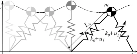
This Section covers both the model and the controller design for the highest abstraction level considered in this work, the V-SLIP model, as presented in [6] and illustrated in Figure 1.

A. V-SLIP model

The V-SLIP model consists of a point mass mlocated at the hip and two massless linear springs with rest lengthL0 and variable stiffnessk0+ui, as illustrated in Figure 1. The

system is furthermore assumed to be planar so the position of the hip is described in the sagittal plane by (x, y). The

control inputs to the V-SLIP model are the variation of the stiffness of the two legsu1 andu2, the rest of the joints are passive.

The system dynamics of the V-SLIP model are given in [6] and written as:

m 0 0 m ¨ x ¨ y + 0 mg0

−Fs0(x, y) =Fsu(x, y) (1)

Wheremis the hip mass,g0is the gravitational acceleration,

Fs0 the total force exerted by the springs on the mass due to

the nominal spring stiffnessk0andFsu the forces exerted on

the mass due to the variable componentui which are control

inputs to the system. The controller described in the next section describes how these control inputs are calculated.

The dynamics of the robot are hybrid in nature, due to the two different phases a step is composed of, i.e. single support and double support. During the single support phase, only one leg can be used to control the hip motion as dynamics of the other leg are not considered at that point. It might happen that a flight phase occurs, when both feet briefly lose contact with the ground. While this should not happen in nominal conditions, we explicitly model such a phase for completeness.

For a walker based on a V-SLIP model it is proven that there exists a control law to make it both robust and energy efficient [6]. This control law is aimed to exploit the natural dynamics of the system so less control effort is required. The robustness is claimed because the leg stiffness can be changed such that a stable gait is recovered after a disturbances has occurred. Figure 1 illustrates the motion of the V-SLIP model for two succeeding steps. The dotted line shows the hip height during the step, it is observed that the lowest position is during double support and the highest position of the hip is during single support when the stance leg is in vertical position.

B. V-SLIP controller

A control strategy for the bipedal V-SLIP model, which renders its dynamics asymptotically stable to an arbitrary gait, is described in [6] and is proven to enhance the robustness of the system.

The V-SLIP controller aims to maintain a certain natural gait, as defined for the bipedal SLIP model by a nominal leg stiffness k0 and spring rest length L0 [4]. Because the horizontal position of the hipxis a monotonically increasing

k

+u

m

L

x y

k

+u

Fig. 1. Walking motion of walker based on the SLIP model with variable stiffness springs

variable, it is possible to parameterize a specific gait by this variable. The reference gait can then be fully described by the hip heighty(x)and the forward hip velocityx˙(x). These two variables are chosen as a reference because they are a measure for a part of the amount of energy associated with the gait, potential energy and kinetic energy respectively. The problem which is solved by the proposed controller in [6] is summarized here as:

Given a desired natural gait, parameterized by

x, as(y∗_(x),x˙∗_{(x)), find control inputsu}

1andu2, such that,

lim

t→∞y(t)−y

∗_{(x(t)) = 0}

and, for some smallε >0,

lim

t→∞|x˙(t)−x˙

∗_{(x(t))|< ε}

i.e., such that the trajectory(x(t), y(t))approaches

the natural gait asymptotically, with bounded error in the desired forward velocity.

From the error in the hip height and the error in the forward velocity, the V-SLIP controller derives the change in leg stiffness u1 and u2, which is added to the nominal stiffness k0 to obtain the total leg stiffness. From the total stiffness the forces which are applied to the hip mass are then calculated as:

Fi= (k0+ui) (L0−Li), i= 1,2, (2)

whereLi is the leg length at that moment in time.

During the single support only one force is acting on the mass while in double support both legs, so two forces acts on the hip mass. During double support the controller thus also calculates two control inputs (u1 andu2), one for each leg.

III. V-SLIPWITH KNEES

K

K

m

m

m

m

Fig. 2. Schematic model of the biped walker—The model features variable stiffness knee joints and its mass distribution is such that it approaches that of the V-SLIP model, depicted in gray.

A. Model

The ‘V-SLIP with knees’ model is shown in Figure 2, in black. This dynamic system consists of four rigid bodies: left upper leg, left lower leg, right upper leg and the right lower leg, for each body the center of mass is indicated, labeled as

mulandmll. It is assumed that the masses of the upper legs

are larger than the lower legs, with a total mass distribution such that the center of mass is close to the hip joint, aimed to closely approach the point mass distribution of the V-SLIP model. Furthermore, it is assumed that each body has a mass distribution similar to that of a solid cylinder. The bodies are connected by means of three joints: the upper legs by the hip joint, and each pair of upper and lower leg by a knee joint. From Figure 2 it is observed that the virtual spring legs of the V-SLIP model (shown in gray) have been replaced by a segmented leg configuration, where the upper and lower leg are connected by torsion springs with variable stiffness. The knee angles are depicted as θi and the angle between

the two upper legs (the hip angle) is depicted asϕ.

B. Stance Leg Controller

The proposed controller for the V-SLIP model calculates via a desired leg stiffness, a desired force generated by the stance leg which is applied on the hip. From Figure 2, it is clear that a conversion between the straight leg configuration of the V-SLIP model and the segmented leg configuration of the biped model is required. In particular, this requires a conversion from the translational stiffness (N/m) and

force (N), to the rotational domain: N m/rad and N m

respectively.

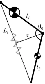
The conversion is visualized in Figure 3. The moment arm

a, which defines the relation between the translational and

rotational domain (τ=a·F), is equal to the shortest distance

between the knee joint and the virtual leg. It can be easily shown that this distance is equal to

a=l1l2

Li

sin(θ),

where l1 and l2 are the lengths of upper and lower leg respectively. The singularity θ = π is avoided by an

end-θ

l

l

L

a

Fig. 3. Visualization of the moment arm of the knee—The V-SLIP model has translational springs as legs. The behavior of these translational springs is mapped onto the behavior of the variable stiffness actuators in the knee joints. The mapping is defined through the moment arma.

stop because otherwise this would lead to a decoupling ofF

andτ because then a= 0.

C. Swing Leg Controller

The motion of the swing leg, in the single support phase, is governed by a motion profile generator. This part calculates the profiles for both the hip and the knee of the swing leg. These motions are parameterized by a variable which is set to

0at the beginning of each step and equals1at the predicted end of that same step.

The motions are designed such that the swing leg is first retracted, then swung forward, and then extended again for touchdown. To achieve the desired motion of the knee joint, the stiffness of the knee joints are controlled to have high stiffness for accurate motion tracking, but the stiffness is lowered just before the predicted moment of touchdown to absorb the impact force.

A software switch selects the correct setpoints during the different phases. By reading the state of a pair of sensors attached to the end of both legs, it is known whether the left leg, the right leg or both legs are touching the ground. From this information the correct control inputs are chosen, i.e. the position control setpoints during the stance phase and the torque control setpoints during stance.

IV. PHYSICAL MODEL AND CONTROLLER

This section describes a third and final model level and corresponding controller for a bipedal robot based on the two levels treated before, including an explanation on how the required variable stiffness in the knee is realized.

A. Physical model

In order to go to a realistic description of a bipedal robot, a 3D model is designed. The 3D model is based on CAD drawings of the robot and constructed using the 3D Mechanics Toolbox of the 20-sim software package [10], and includes full 3D dynamics, ground contact models, and actuator dynamics. For this design, an upper leg mass of

Fig. 4. Visual representation of the robot model—The model is imple-mented using the CAD drawings of a robot design, and includes full 3D dynamics and ground contact models.

leg length of1m (maximally stretched knee). The sideways

motion of the robot is constrained by a guide rail in order to keep the motion of the robot in the sagittal (2D) plane. A visual representation of the modeled robot is depicted in Figure 4 (the guide rail is not shown).

The required variable leg compliance of the biped model is reproduced in the 3D model by means of variable stiffness actuators in the knees. This class of actuators are character-ized by the property that they can change the output position and stiffness independently. By using these actuators in the knee joints of the robot, the variable leg stiffness behavior of the bipedal V-SLIP model can be reproduced.

F

d

q

k

k

d-q

x

Fig. 5. Working principle of variables stiffness actuator. The pivot moves along the lever, thus changing the ratio of the lever.

B. Variable Stiffness Actuator

In this work, we choose to use the vsaUT-II actuator [11]. The vsaUT-II uses the concept of a lever with a moving pivot, as is shown in Figure 5. Considering two springs with a fixed stiffness kand a lever length d, the apparent output

stiffness K is:

K(q1) =∂F

∂x =

q1

d₋q1 2

·2·k

where q1 is the position of the pivot. This method enables a zero stiffness configuration and a rigid configuration. For

q1= 0,K equals zero and forq1=d,K is infinite. Besides q1 the vsaUT-II has a second degree of freedom, denoted byq2, which defines the equilibrium position of the

output. The torque delivered by the actuator at the output is a function of the state of the internal spring element, the output position θ, and the two internal degrees of freedom

q1 andq2.

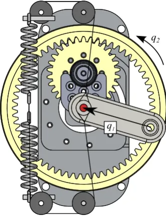
A CAD drawing of the vsaUT-II is shown in Figure 6. In the figure a planetary gear system is observed, the gears are chosen such that the pivot moves in a straight line along the lever.

q2

q1

Fig. 6. CAD drawing of a slightly adapted version of the vsaUT-II. This design has been implemented in the bipedal robot.

C. Physical model controller

Because of the constraints on the robot by means of a guide rail, the biped can still be assumed to be planar, so the control law from Section III (the ‘V-SLIP with knee’ model) is still applicable. Because the previous models assumed an ideal variable compliant knee element and no VSA, the control of the VSA needs to be added to the previous presented controller.

The output of the controller of Section III is a required knee torque together with a desired knee stiffness. These two variables will be the inputs to the VSA controller which calculates the required motion for both degrees of freedom of the actuator. This controller is based on the controller presented in [12].

Given the desired knee torque τd, and given the exerted

torqueτ from the vsaUT-II model [11], we define a desired

rate of change

˙

τd=κp(τd−τ), (3)

for some κp > 0. The rate of change of the output torque

delivered by the VSA can be shown to be of the form

˙

τ =Vq

˙

q1

˙

q2

+Vθθ˙ (4)

where the matrix functionVq and scalar function Vθ follow

from the VSA mechanism design [11] and _θ˙ _{is the rate of}

In order to find the required ( ˙q1,q˙2) to realize τ˙d, (4)

needs to be inverted. HoweverVq is not square, causing the

problem to be under-constrained. To resolve the redundancy, [12] proposes to introduce a weighted pseudo inverse with a dynamic weighting:

V]

q =M−1VT V M−1VT

−1

(5) With M:

M =

w1 0

0 w2

(6)

where w1 and w2 are functions of q1 and q2 respectively. The purpose of the weighting functionswi is to control the

ratio betweenq˙1andq˙2, and are constructed to appoint near-infinite weight to a degree of freedom approaching its ex-tremal positions. Since, in the vsaUT-II, the motor controlling

q1is much smaller than the motor controllingq2, the former is given a higher weight, to prevent overloading of the motor. However, q1 is allowed to reach the maximum stiffness position, as this might be required to reject disturbances.

Given the pseudo inverse (5), (4) can be inverted, yielding

˙

q=Vq]

˙

τd−Vθθ˙

+g(Kd)

The function g(Kd) is a special function that regulates the

VSA output stiffnessK to the torsional equivalentKd ofk0 in the null-space ofV, i.e. it attempts to keep the virtual leg

stiffness close to k0 without interfering with effectuation of

τd (see [12] for details).

V. THREE LAYER CONTROL STRUCTURE

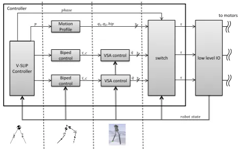
The former sections covered three iteration steps of mod-eling and control a bipedal robot. The controllers from these sections together form a complete controller for the 3D biped model, the way these parts are connected is shown in Figure 7.

The V-SLIP controller shown on the left, maps the robot state on the V-SLIP model and calculates leg stiffness variations for the V-SLIP model. Then, in a second layer, these stiffness variations are mapped onto the knees of the bipedal model and along with this control, trajectories for the swing leg and hip trajectory are calculated. At the physical level, the VSA control maps the desired knee torques during stance onto the individual degrees of freedom of the vsaUT-II. After this part the aforementioned switching block selects the correct control inputs for the different joints, e.g. stiffness control during the stance phase and motion control during the swing phase. The low level IO block takes care of the required motor currents in order to achieve the desired torques or motions.

VI. SIMULATIONS

In this Section, numeric simulation results are presented that validate the control strategy. For the simulations the 3D model from Section IV is used, together with the complete control structure as summarized in Section V.

In Figure 8, the top plot shows the vertical positionyof the

hip during walking, together with the referencey∗ obtained

Controller VSA control V-SLIP Controller VSA control Motion Profile

switch low level IO

𝑟𝑜𝑏𝑜𝑡 𝑠𝑡𝑎𝑡𝑒 𝜏 𝜏 𝜏 𝑞 𝑞 𝑞1, 𝑞2, ℎ𝑖𝑝

𝑝ℎ𝑎𝑠𝑒

𝜏 , 𝑐

𝜏 , 𝑐 𝑝 2 2 3 to motors Biped control Biped control

Fig. 7. Multi-layer control architecture—From left to right, the first layer maps the robot state onto the conceptual V-SLIP model. The control signals that are calculated for this model are then mapped to the ‘V-SLIP with knee’ model. The third level maps these torques onto the control of the variable stiffness actuators. A low-level controller switches between stiffness control in stance phase and motion control during swing.

from the SLIP model. It can be seen that in steady state conditions, the height of the robot deviates approximately a centimeter from the reference of the conceptual SLIP model. The lower plot shows the forward velocity x˙ of the hip,

together with the reference x˙∗. The spikes are caused by

the impact of the feet with the ground. It is observed that the velocity is out of phase with the reference. This is due to the dynamics of the swing leg, which need to be swung forward during the single support phase. These dynamics not included in the V-SLIP model and therefore not present in the reference trajectory. The motion of the inertia of the swing leg causes extra acceleration and deceleration of the hip. Despite the velocity and hip height deviations of the bipedal robot a stable gait is obtained using a controller which is mainly based on the simple V-SLIP model.

The hip and the knee motion during four steps are shown in Figure 9, to illustrate the switching between VSA control and motion control. The hip angleϕshows a smooth periodic

motion, representing the hip swinging forward and backward during subsequent steps. The motion of the knee angles is shown in the center plot. During the swing phase the knee is controlled to an angle θ = 2.0 rad, retracting the leg to

avoid foot scuffing. Before ending the swing phase, the knee angle is controlled toθ= 2.86rad, extending the leg to its

full length just before impact. During the stance phase, the knee is passively compressed to an angleθ≈2.5 rad.

All graphs show a certain asymmetry between the left and the right leg. There are two possible explanations for this. One explanation is the initial configuration of the biped: during the very first step the right leg is chosen to be the leading leg, which might cause the asymmetry. Another cause might be that the guide rails constraining the sideways motion of the robot, are mounted at the top left side of the left leg, thus introducing an asymmetry.

VII. ROBOTDESIGN

0 5 10 15 0.92 0.94 0.96 0.98 1 time (s) y (m ) y y∗

0 5 10 15

0 1 2 3 time (s) ˙ x (m /s ) ˙ x ˙ x∗

Fig. 8. Simulation results—The top plot shows the hip heightyof the bipedal robot, plotted along with the referencey∗_{(x). The lower plot shows the}

forward velocityx˙of the hip plotted along with the referencex˙∗_{. It can be seen that a stable gait is attained.}

10.5 11 11.5 12 12.5 −1 −0.5 0 0.5 1 time (s) h ip an gl e ϕ

10.5 11 11.5 12 12.5 2 2.5 3 time (s) kn ee an gl e θ

10.5 11 11.5 12 12.5 2000 4000 6000 8000 time (s) li n ea r st iff n es s N/ m

Fig. 9. Hip and knee angles during simulation—The top plot shows the sinusoidal hip motion, swinging forward and backward. The center plot shows the knee angles for both the left and right leg. The lower plot shows the calculated virtual leg stiffness, as defined in the V-SLIP model.

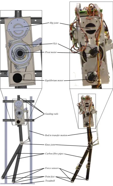
robot is depicted. On the left is a CAD view and on the right is a photograph of the realized robot. In the center the most important features are indicated. In this section several aspects are discussed in more detail.

A. Design

The designed robot features different properties which are required to match the original V-SLIP model as close as possible. For the V-SLIP model only contains a point mass at the hip, it is required that most of the mass of the robot is situated close to the hip joint. To meet these weight distribution requirements the upper and lower leg parts are made out of light-weight carbon fiber tubes. Also

the variable stiffness actuator, which acts on the knee joint, is situated close to the hip joint. A light-weight transmission rod connects the output of the variable stiffness actuator to the knee joint. Figure 10 presents both the CAD model of the biped and a photograph of the constructed biped, furthermore the most imported features are indicated.

The actuation of the knee is transferred from theq2motor to the frame of the variable stiffness actuator by a timing belt which can be tensioned by moving the mounting plate of the q2 motor. To transfer the movement of the output of the VSA to the knee joint, a pulling rod is used. This consists of a stud with ball joints at the ends, to prevent a static over defined construction.

The left and right leg are connected by an actuated hip joint. The hip joint consists of one pipe rotating inside another, where the inner pipe is fixed to the left leg and the outer pipe is fixed to the right leg. An Oldham coupling is placed between the output shaft of the motor, which is mounted in the inner pipe, and the outer pipe to prevent a static over defined construction.

In order to constrain the motion of the robot to be only in the sagittal plane a set of linear guides is mounted and connected to the left leg via a passive joint.

B. Electronics and software

Hip joint

VSA

Pivot motor

Equilibrium motor

Guiding rails

Rod to transfer motion

Knee joint

Carbon fibre pipes

Force sensors

Point feet Treadmill

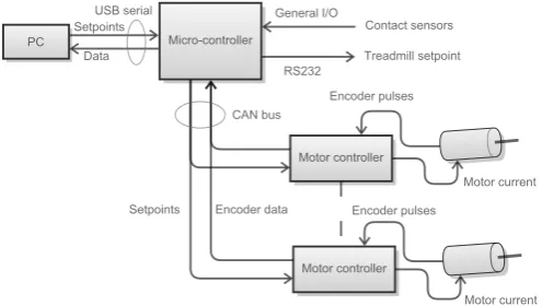
send to the PC via the RS232 protocol over the USB connec-tion. In parallel the set points generated by the controller are received by the MBED and translated to set points for the different motors. These set points are applied to the specific motor via a dedicated third party motor controller of ELMO. The complete controller is implemented on a PC by means of a Simulink model. Each time step this model receives new setpoints from the robot and calculates new setpoints accordingly. The model is executed as a Real Time Target so a real time control loop is achieved using a normal PC.

Micro-controller Motor controller Setpoints Data Contact sensors Treadmill setpoint Motor controller USB serial CAN bus Encoder data Setpoints RS232 General I/O Encoder pulses Encoder pulses Motor current Motor current PC

Fig. 11. Schematic overview of the electronics. The main controller is realized in Simulink on the PC. The low level control and IO is done by the micro controller and the motor controllers.

C. Sensors

To determine the lift off and touch down events for the feet, a pressure sensor is used. This pressure sensor works as a variable resistor, having a high resistance when no pressure is applied and a low resistance when a high pressure. By enclosing this variable resistor in a voltage divider an analogue signal that resembles the pressure is generated. Since only a boolean signal is required, i.e. contact or no contact, a Schmidt trigger generates an on/off signal with hysteresis to avoid bouncing effect. The circuit with the Schmidt trigger is located at the feet to avoid the analog signal to distort.

To measure the angles of the joints, relative optical en-coders are used. The actuated joints have an encoder on the motor, the passive joints are equipped with a separate encoder placed directly on the specific shaft. In total there are eight optical encoders, two on the equilibrium motors, two on the pivot motors, two on the knee joints, one on the hip motor and one on the joint between the robot and the supporting frame. The optical encoders are interfaced via the motor controllers, which support two encoders each. With a simple command the actual position and the actual velocity for each encoder can be acquired. Because relative encoders are used, it is required to calibrate all joints before the walking control is started.

VIII. EXPERIMENTS

This section describes the experiments which are per-formed using the controller as presented before, implemented on the designed robot as described in Section VII.

Figure 12 shows the two variables of the biped which are used to track a desired reference, e.g. the hip heightyand the forward velocity of the hipx˙. These two variables are plotted in black whereas the reference trajectories are shown in gray. The figure shows 5 seconds of a performed experiment, from this experiment it is observed that the hip height is going to the correct periodic motion, but the absolute height is decreasing over time so the error in comparison to the reference is increasing. From the forward velocity it is observed that the reference trajectory is badly tracked, high and low peaks are observed, but the average velocity of the hip stays in the same order of magnitude as the desired velocity.

108 109 110 111 112 113

0.88 0.9 0.92 0.94 0.96 0.98 1 time (s) y (m )

108 109 110 111 112 113

−0.5 0 0.5 1 1.5 2 time (s) ˙ x (m /s )

Fig. 12. Experimental results — The top plot shows the hip heighty in black during seven succeeding steps of the robotic biped, in gray the desired hip height is shown. The lower plot shows the forward velocityx˙ of the

hip, also with its corresponding trajectory in gray. It is observed that both trajectories are badly tracked but that the robot is able to walk for seven steps autonomously

rad. However it is observed that the knee angle during stance, is decreasing in succeeding steps.

108 109 110 111 112 113

−1 −0.5 0 0.5 1 time (s) h ip an gl e ϕ

108 109 110 111 112 113

1.8 2 2.2 2.4 2.6 2.8 3 time (s) kn ee an gl e θ

Fig. 13. Experimental results — The top plot shows the hip angle swinging forward and backward during walking. The lower plot shows the matching knee angles, in gray the left leg and in black the right leg. During swing the leg is retracted to a knee angle of approximately 2 rad and during stance the knee angle is approximately 2.4 rad but decreasing.

From both figures presented in this section it is observed that the height of the robot is decreasing during succeeding steps. This is due to a combination of different mechanical and software issues. Because of the chosen implementation it was not possible to use the same high gains throughout the controller as the gains used during simulation. The desired gains led to unstable behavior which might be due to a too large loop time of the implementation. Another issue is that the motor actuating theq2motion of the VSA, cannot deliver enough torque which is required to achieve fast setpoint tracking. The apparent bad tracking of the forward velocity might be due to the fact that the velocity of the hip is not measured directly, but is derived from the velocities of the different joints. As this calculation requires multiple encoder velocities, multiple entry points for noise exist. Furthermore the forward velocity is only controlled when both legs touch the ground (double support), as this is only the case for a small amount of time compared to the duration of single support, less control effort is put into the tracking of the velocity error than into the hip height tracking.

IX. CONCLUSIONS

This paper presented a realistic model, a controller and a design of a bipedal robot which features variable compliant actuators. A multi-layer control strategy was designed in order to control the different degrees of freedom of the robot. The high-level control is based on the conceptual V-SLIP model and calculates stiffness setpoints for the virtual legs. A second layer of the controller maps the control inputs of the V-SLIP model onto the model where knees are incorporated. The final layer controls the different degrees of freedom of the VSAs. By means of this layered controller design all intermediate steps are relatively simple and therefore easy to implement. The performance of the controller was demonstrated by simulations and experiments. The simula-tions showed that the controller is capable of maintaining a specified gait for the realistic model, a long period of time. Even while a large part of the controller is based on the simple V-SLIP model which does not incorporate leg inertia’s and swing leg behavior. The experiments show that the biped is capable of making a few succeeding steps without human assistance proving that the designed controller architecture is fundamentally capable of letting the robot walk. However there are still some issues with both the implementation of the controller and some mechanical parts which now prevent the robot from maintaining a certain gait.

Future work should solve the mentioned issues so the robot is capable of maintaining a specific gait for a long period of time. If that has been done, it should be investigated to what extend the robot is capable of dealing with disturbances. Furthermore it might be interesting to investigate whether it is possible to walk using a different nominal leg stiffness, and as a next step also to make gait transitions during walking.

ACKNOWLEDGMENT

The authors would like to thank Wouter de Geus for his contribution to the design and construction of the bipedal robot.

REFERENCES

[1] T. McGeer, “Passive dynamic walking,” International Journal of Robotics Research, vol. 9, no. 2, pp. 62–82, 1990.

[2] S. Collins, A. Ruina, R. Tedrake, and M. Wisse, “Efficient bipedal robots based on passive-dynamic walkers,”Science, vol. 307, no. 5712, pp. 1082–1085, 2005.

[3] Boston Dynamics, “PETMAN - BigDog gets a big brother,” online: http://www.bostondynamics.com/robot petman.html, 2011.

[4] H. Geyer, A. Seyfarth, and R. Blickhan, “Compliant leg behaviour explains basic dynamics of walking and running,”Proceedings of the Royal Society B, vol. 273, no. 1603, pp. 2861–2867, 2006. [5] J. Rummel, Y. Blum, and A. Seyfarth, “Robust and efficient walking

with spring-like legs,”Bioinspiration and Biomimetics, vol. 5, no. 4, p. 046004, 2010.

[6] L. C. Visser, S. Stramigioli, and R. Carloni, “Robust bipedal walking with variable leg stiffness,” inProceedings of the IEEE International Conference on Biomedical Robotics and Biomechatronics, 2012. [7] G. Garofalo, C. Ott, and A. Albu-Sch¨affer, “Walking control of fully

actuated robots based on the bipedal slip model,” inProceedings of the IEEE International Conference on Robotics and Automation, 2012. [8] B. Vanderborght, R. van Ham, D. Lefeber, T. G. Sugar, and K. W.

[9] VIACTORS, “Variable Impedance ACTuation systems embodying advanced interaction behaviORS,” http://www.viactors.org, 2012. [10] Controllab Products B.V., “20-sim,” online: http://www.20sim.com,

2012.

[11] S. S. Groothuis, G. Rusticelli, A. Zucchelli, S. Stramigioli, and R. Car-loni, “The vsaUT-II: a novel rotational variable stiffness actuator,” in Proceedings of the IEEE International Conference on Robotics and Automation, 2012.

12 MSc report - J.G. Ketelaar

3 Conclusion and recommendations

In addition to the conclusion as drawn in the presented paper, this chapter covers a general conclusion on the complete master project and furthermore gives a couple of recommenda-tions for future work.

3.1 Conclusion

This work was a follow up on the work of Wouter de Geus, who designed the bipedal walker and proved the concept by means of a simple controller. The goal of this project was to design a new, more advanced, controller in order to benefit of all the properties the bipedal walker provides. The controller as presented in this work is a flexible multi-layer controller which is capable of controlling all degrees of freedom of the robot such that the robot can maintain a certain gait during simulation, and is capable of making a couple of autonomous steps during experiments.

During the project it became evident that a walking pattern is a really complex motion and in order to make robots walk like humans, a complex controller is required. Before such robots will come into existence more research effort should be put into bipedal walking robots, espe-cially on how to control such robots. This report has covered a piece of this research and the results can be used as a starting point for future research on this topic.

3.2 Recommendations

For future work the following topics should be considered.

3.2.1 Constant rotational stiffness gaits

From the different experiments it was found that it is hard to adjust the rotational stiffness of the VSA during a stance period. When a large load is applied on the output of the VSA, i.e. the weight of the robot during the stance phase, a large force is required for the pivot to move to a more stiff position. In contrast to the stance phase, during the swing phase, no load is applied on the VSA and it is thus fairly easy to adjust the stiffness. Therefore it is interesting to search for possible stable gaits by using a constant rotational stiffness instead of a constant (virtual) linear stiffness. When such gaits exists, the correct stiffness can be applied during the swing phase and is benefited during stance.

3.2.2 Simple controller

The controller proposed in this work features three different levels and a lot of different gains and is therefore highly flexible but also quite complex. This approach works in theory for the designed model, but in practice the controller might still be too complex. In order to achieve a nice walking behavior of the designed bipedal robot, it might be good to look into a con-troller which is less flexible but explicitly designed for the existing biped and therefore easier to implement and tune.

3.2.3 Passive damping

During the experiments it was observed that the robot needs to cope with large forces at the moment of impact of the feet. These forces results in large disturbances during the walking, which particularly disturb the forward velocity of the robot. By adding a passive damper at the end of the feet, the impact forces can be absorbed for a vast amount. Such a damper can be realized by a piece of rubber material, which also increases the grip of the feet on the floor, the lack of grip turned out to be a problem sometimes during the experiments as well.

13

A Manual

This chapter describes all steps required in order to work with the bipedal robot and the de-signed controller. It is emphasized that this manual is an extension to the manual described in (de Geus, 2012). Specifically, section A.1 of this report replaces section 4.1 of the mentioned report and section A.3 replaces section 4.5 of that same report.

A.1 Quick user guide

To give a demo with the biped walker you’ll have to follow the procedure as described in this section. It is assumed here that everything is working properly. If not, look in the troubleshoot section.

Preparations

• Boot the PC (labeled VSA-II) and log in with password ’ram’.

• The robot has to be hoisted so the legs can move freely without touching the treadmill. The robot is attached to a set of pulleys that lead to a cable with which the robot can be lifted. This cable can be fixed to the handlebar of the treadmill with a clove hitch.

• The position of the joints is not important since the homing procedure will take care of this.

Start up

• Launch Matlab and navigate to the directory where the ’serial_com.m’ file is located. • Power up the system by unlocking the emergency button.

• Check if the switch on the main board is in ‘Controlled mode’. • Wait for the treadmill to power up until it beeps.

• Execute the ’serial_com.m’ script to open a monitor window. • Now reset the MBED by pressing the pushbutton on the MBED.

• In the monitor the following message should appear: ‘MBED Device with LPC1768 (100.00 MHz)’ followed by ‘Start-up complete, waiting for INIT command. . . ’. If this message does not show up, reconnect the usb cable and rerun the ’serial_com.m’ script.

Figure A.1:Matlab monitor window

14 MSc report - J.G. Ketelaar

Initialization and homing

• Press ‘Initialize’.

• Now all motor controllers and the treadmill are initialized.

• The following message should appear: ‘Initialization complete, waiting for HOME com-mand. . . ’.

• Now press ‘Home’ to start the homing procedure.

• The homing process is mainly autonomous, but you should check if everything goes cor-rect.

The following should happen:

• The pivot of the VSA moves to the zero stiffness position.

• The VSA frame rotates until the leg is fully stretched and the output of the VSA touches the VSA frame.

• The VSA frame rotates 60 degrees in opposite direction. • The pivot moves to the infinite stiffness position. • The VSA frame rotates until the leg is fully stretched.

After both legs are homed the hip joint will be homed. The system will count down 5 seconds. You should move the hip parts parallel using T-shaped tool and hold it until the homing is completed.

Figure A.2:Use the T-shaped tool to perform the hip homing.

Starting

• Press ‘Start’ in the monitor application.

• The robot will move one leg forward and the other backward.

• Now the robot can be lowered so it stands. Release the clove hitch to lower the robot. When the robot is standing on the treadmill, create some slack in the cable and then fix the cable to the handle bar again with a clove hitch. In case the robot falls during walking it is caught by the cable.

• Wait for 20 seconds, the robot will home the frame-angle and takes its initial configura-tion.

• When the green led turns on, the robot is waiting for setpoints from the PC. Now lift the robot and start the treadmill manually to the desired velocity.

• Check whether the communication is still running, otherwise reconnect and restart the Simulink model.

• If the communication is up and running you can slowly lower the robot till it touches the treadmill and start walking.

Walking

To start walking the robot needs help, it does not start walking autonomously. Make sure the emergency button is within reach of your hand or foot. When the robot is standing on the

APPENDIX A. MANUAL 15

treadmill, grab the robot by either the right pulling rod or the right part of the hip joint. Pay attention that you hold the robot correctly! Make sure there are no fingers between the hip joint or near the VSA.

When the robot start walking, assist the robot making its first steps. After a few steps you can carefully release the robot, but the chance that the robot stumbles is always there. When the robot stumbles, either hoist the robot or push the emergency button. When the button is pushed you should redo the whole process from step one, including the homing procedure. When the robot is only hoisted, you can immediately try again to let the robot walk.

A.2 Troubleshooting

In this section the most common problems and malfunctions are discussed. In any case some-thing fails it is always good to check the wiring and to check if everysome-thing is powered up as it should. This troubleshoot section is an extension to the troubleshoot section as given in (de Geus, 2012). If the specific problem is not mentioned in this section, the troubleshoot sec-tion of the other report should be checked.

The communication with Simulink is lost

It happens often that when the treadmill is turned on, the serial connection between the biped and the Simulink model is lost. Somehow the treadmill generates a lot of noise in the usb cable when it starts. When this happens, hoist the robot, reconnect and restart the Simulink model and check whether the communcation is up and running again. If that is the case the robot can be lowered again.

The Matlab user interface doesn’t start

When the Matlab script cannot make a serial connection to the biped, the script stops and prints "Failed!" on the Matlab commandline. Make sure that the usb cable is connected and if thats the case, try to reconnect the cable and run the script again.

MBED doesn’t respond

Check if the MBED started correctly. There should be a LED blinking. If not, first reset the MBED and check again. If there is still no LED blinking, the binary file might not be properly loaded. Recompile the code and copy the binary file to the MBED. Normally the binary file is automatically copied to the MBED after compiling. After copying a binary file to the MBED, always restart the device by a reset or a powercycle. When the LED does blink but still there is no reaction of the biped when ‘Initialise’ has been pressed, reconnect the usb cable, kill the Matlab process by pressing Ctrl+C and run the script again.

Treadmill doesn’t beep

If the treadmill does not beep, does not make any sound and nothing is on the display it is most likely that it does not have power. Check if the power cord is connected, the power switch is switched to ON and that the emergency button is unlocked.

Initialisation fails

There are two possible reasons for the initialization to fail. Either the treadmill is not respond-ing or one or more motor controllers does not respond. For both check the power wirrespond-ing and the signal wiring and the biped.

The homing procedure doesn’t go as it should

Check if all wires are connected correctly. Especially check the motor wires and the encoder wires. If a change has been made to the homing procedure, check the code.

16 MSc report - J.G. Ketelaar

When the robot should start walking it collapses

This might also have two reasons. There is a hardware switch on the robot which can be in controlled, and in manual mode. This latter mode is intended for debugging and it might be the case that no setpoints will be commanded to the motor controllers when the switch is in this mode. The manual mode is only intended for single command motions to the motors. This can be needed for experiments. For normal walking the mode switch should always be in ‘Controlled mode’. Another reason for the robot to collapse is that the communication beteen the robot and Simulink has been lost. In that case hoist the biped, and restart the Simulink model. In the ‘Serial receive’ block it can be checked whether the communication is ok.

A.3 Software

This section describes the software which is used on both the host PC and the robot itself. It should be read as a replacement for section 4.5 of (de Geus, 2012). The software for this project consists of two parts, the part which runs on the robot, written in C code, and the part on the PC running in Matlab and Simulink.

A.3.1 MBED software

The NXP MBED micro-controller features a powerful ARM processor and a lot of different in-and output ports. NXP offers an online development environment but as this method re-quires an internet connection an offline C library was used. This library is specially written for this project and is available as an opensource project on http://code.google.com/p/mbed-lib/. Most of the software for the MBED device is already covered in the Master thesis of W. de Geus, however in this project the control of the biped is no longer controlled by the MBED but by a PC. Therefore the MBED sends a data packet over the serial bus at 100Hz, which contains the complete state information of the robot. Also at 100Hz, the device receives new setpoints from the PC which are applied to the motors by means of the motor controllers. To make sure that all packets are received in time and no buffer overflow occurs, a interrupt handler is writ-ten for the serial port. This piece of software is executed each time a byte is received at the serial input port and takes care that the bytes is copied to a larger buffer. This buffer is polled at 100Hz as described before.

A.3.2 PC software

The complete three layer control structure as is described in both papers presented in this re-port, is implemented using Matlab and Simulink. A Matlab script takes account of the user interface which is required for the initial interaction with the robot like sending the homing and start commands. A Simulink model, executed as a Real Time Target, is used for the actual control of the robot during walking.

Matlab script

The main part of the this script exists of an infinite loop which continuously listens to the serial port. In the mean time different callback functions, binded to the user interface buttons, can send a command to the robot over the serial bus when such a button is pressed. Once the start button has been pressed, the robot takes its initial configuration and waits for floor contact. Once this is realized, the robot sends a ’Go’ command to the Matlab script, when the script receives this command it closes its own COM port connection, launches Simulink and sends an execute command to the Simulink model.

Simulink model

The Simulink model is used during the actual control of the robot during walking, so after it has received the Start command. The model is a discrete time model and is executed as a

APPENDIX A. MANUAL 17

Figure A.3:The top view of the Simulink model

Real Time Target which means that it has almost direct access to the PC’s resources without interference of the Operating System. Therefore it is possible to send, receive and solve all model equations each time step of 0.01 seconds (100Hz) The top view of the Simulink model is shown in Figure A.3, this view consists of three parts, the serial receive block, the controller, and the serial send block.

The controller is shown in Figure A.4. The left most block is the V-SLIP controller which calcu-lates from the robot state the desired linear stiffness and the desired force along the virtual leg. These signals go to the next block which convert the linear desired values to their equivalent rotational desired values, e.g. the ‘V-SLIP with knees’ controller. The output signals of these blocks are a desired rate of change of the knee torque and a desired rotational stiffness. The third stage contains both the trajectory generator for the swing leg, and the VSA controller. The latter block calculates the desired velocities for the degrees of freedom of the VSA in order to achieve the desired rate of change of the output torque. The final ‘switching block’ selects the correct signals for the different actuators, i.e. the swing leg position setpoints during swing and the VSA controller velocity setpoints during stance. Furthermore this block contains a few sim-ple PD-controllers in order to calculate a desired torque for the motors based on the different position and velocity setpoints.

18 MSc report - J.G. Ketelaar

Figure A.4:The controller of the Simulink model

Controller design for a Bipedal Walking Machine

using Variable Stiffness Actuators

J.G. Ketelaar, L.C. Visser and R. Carloni

Abstract— The bipedal spring-loaded inverted pendulum (SLIP) model is known to resemble human walking to a large extend, and it is therefore used extensively to study human-like walking. The extended variable spring-loaded inverted pendulum (V-SLIP) model provides a control input for gait stabilization for the SLIP model. However, these models are purely conceptual, as they assume massless legs. This work presents a control strategy that essentially maps the conceptual V-SLIP model on a realistic model of a bipedal walker. This walker implements a variable compliance in the knees in order to exploit the benefits of a varying leg stiffness during walking. In particular, the knees are actuated by variable stiffness actuators (VSAs), which allow the knee angle and its stiffness to be controlled independently. The proposed controller consists of multiple levels, mapping the control of the walking gait onto the control of the degrees of freedom of the VSAs. Using numeric simulations, the controller design is validated.

I. INTRODUCTION

The human musculoskeletal system enables highly energy efficient and robust walking. However, walking machines are not yet close to achieving similar performance with the same level of robustness. In particular, robotic walkers are either energy efficient, such as passive dynamic walkers [1], [2], or robust, such as PETMAN [3]. In order to be able to build robotic walkers that can come close to human performance levels, a better understanding of human walking is needed.

Human-like walking can be modeled by a dynamic system composed of a mass and two massless springs, acting as legs. This bipedal Spring-Loaded Inverted Pendulum (SLIP) model reproduces, to a large extent, the human hip motion and ground reaction forces observed in human gaits [4]. As shown in [5], the stiffness of the legs not only influences the type of gait, but also robustness against external disturbances. This property inspired the introduction of the bipedal Variable Spring-Loaded Inverted Pendulum (V-SLIP) model, in which the leg stiffness can be continuously varied [6]. It was shown that a controller exists that, by active variation of the leg stiffness, renders an arbitrary gait asymptotically stable, thus further improving the robustness.

The main shortcoming of the bipedal SLIP and V-SLIP models is that they are purely conceptual. In particular, any robotic walker will be influenced by swing leg dynamics and energy losses due to foot impacts, which have not been incorporated in these models. In [7], it was shown that it is possible to use the passive gait of the bipedal SLIP model

This work was partly funded by the European Commission as part of the VIACTORS project under grant no. 231554.

The authors are with the MIRA Institute, Department of Elec-trical Engineering, University of Twente, The Netherlands. E-mail: [email protected],{l.c.visser,r.carloni}@utwente.nl

onto a fully actuated bipedal robot model by projecting the bipedal SLIP dynamics onto the robot dynamics.

In this work, we present a realistic model of a bipedal walking robot, actuated by variable stiffness actuators [8], [9], a class of actuators that allow the actuator output position and stiffness to be controlled independently. This makes it possible to realize a robot with controllable leg compliance, so that it more closely matches the bipedal V-SLIP model.

Furthermore, a control strategy is proposed that maps the control of the V-SLIP model, presented in [6], onto the VSA control and hip motion control of the biped. The effectiveness of the control strategy is demonstrated by numeric simulation of a physically realistic simulation model.

This paper is organized as follows: Section II describes the model of the robot with its components. Section III covers the design and analysis of the controller and Section IV presents numeric simulation results. The discussion and conclusions are in Section V.

II. MODEL DESCRIPTION

The planar robot walker considered in this work aims to closely resemble the bipedal V-SLIP model presented in [6]. The model and its resemblance to the V-SLIP model are depicted in Figure 1, where the V-SLIP model is shown in a lighter gray shade. The variable leg compliance of the V-SLIP model is reproduced in the robot model by means of variable stiffness actuators in the knees. The VSAs have two internal degrees of freedom, defining an equilibrium output position and the output stiffness respectively. The knee

angle θ can thus indirectly be controlled by the VSA

equi-librium angle and the output stiffnessK. In this Section, we

describe the model in more detail and analyze its dynamics.

A. Model of the Robotic Biped

The model of the robotic biped, as shown in Figure 1, consists of four rigid bodies: left upper leg, left lower leg, right upper leg and the right lower leg. For each body,

labeled as mul and mll, the center of mass is indicated.

It is assumed that the masses of the upper legs are larger than the lower legs, with a total mass distribution such that the center of mass is close to the hip joint, with the aim of approaching the point mass distribution of the bipedal V-SLIP model. Furthermore, it is assumed that each body has a mass distribution similar to that of a solid cylinder. The bodies are connected using three joints: the upper legs by the hip joint, and each pair of upper and lower leg by a knee joint.

CONFIDENTIAL. Limited circulation. For review only.

K

K

m

m

1

m

2

m

θ

θ

x

y _φ

Fig. 1. Schematic model of the biped walker—The model features variable stiffness knee joints and its mass distribution is such that it approaches that of the V-SLIP model, depicted in gray.

The dynamics of the robot are hybrid in nature, due to the foot lift-off and touchdown events throughout a walking gait. In particular, we consider three specific domains. When both feet are in contact with the ground, the robot is said to be in ‘double support’, both legs can then be used to control the hip motion of the biped. When only one foot is in contact with the ground, the robot is said to be in ‘single support’. During this phase, only one leg can be used to control the hip motion, while the other one swings forward. It might happen that a flight phase occurs, when both feet briefly lose contact with the ground. While this should not happen in nominal conditions, we explicitly model such a phase for completeness.

B. Actuation

As already stated, the knees of the biped are actuated by variable stiffness actuators. This class of actuators are characterized by the property that they can change the output position and stiffness independently. By using these actuators in the knee joints of the robot, the variable leg stiffness behavior of the bipedal V-SLIP model can be reproduced.

In this work, we choose to use the vsaUT-II actuator [10]. In this particular actuator design, the change in stiffness is achieved by a variable transmission ratio between an internal spring element and the output. At one extrema of this ratio, the output is infinitely stiff (limited by the stiffness of the mechanical construction), and in the other extrema the output is infinitely compliant (i.e., zero stiffness).

The vsaUT-II has two internal degrees of freedom. The

first one, denoted byq1, defines the output stiffness, and the

second one, denoted byq2, defines the equilibrium position

of the output. The output torque is a function of the state

of the internal spring element, the output positionθ, and the

two internal degrees of freedomq1 andq2.

The internal degrees of freedom of the two VSAs and the

hip motionϕare all controlled by stiff actuators.

III. CONTROLLERDESIGN

The goal of the control strategy presented in this work is to map the control of the bipedal V-SLIP model onto the

controller 𝑠𝑤𝑖𝑛𝑔 𝑠𝑒𝑡𝑝𝑜𝑖𝑛𝑡𝑠 VSA control V-SLIP controller

lin to rot VSA control motion profile

switch low level IO

𝑟𝑜𝑏𝑜𝑡 𝑠𝑡𝑎𝑡𝑒 𝑝ℎ𝑎𝑠𝑒

𝑝

lin to rot 2

2 3

to motors

𝑞 ∗

𝑞 ∗

Fig. 2. Multi-layer control architecture—From left to right, the first layer maps the robot state onto the conceptual V-SLIP model. The control signals that are calculated for this model are then mapped onto the control of the variable stiffness actuators. A low-level controller switches between stiffness control in stance phase and motion control during swing.

VSA and hip motion control of the robot. For this purpose, a multi-layer controller has been designed. The first layer maps the robot state on the V-SLIP model and calculates leg stiffness variations for the V-SLIP model. Then, in a second layer, these stiffness variations are mapped onto the control of the individual degrees of freedom of the variable stiffness actuators. This second layer is also responsible for generating motions of the swing leg during the single support phase. The third, low-level, layer is responsible for the control of each individual degree of freedom, and switches between stiffness control during the stance phase and motion control during the swing phase.

Figure 2 presents a schematic overview of the control architecture, which will be elaborated in further detail in the remainder of this Section.

A. High level controller

At the first layer the biped is assumed to be a simple dynamic structure consisting only of one mass and two vari-able stiffness linear springs, i.e. the bipedal Varivari-able Spring-Loaded Inverted Pendulum (V-SLIP) model, as illustrated in Figure 1.

A control strategy for the bipedal V-SLIP model, which renders its dynamics asymptotically stable to an arbitrary gait, is described in [6] and is proven to enhance the robustness of the system. Because the biped described in this work is assumed to be designed to closely resemble the V-SLIP model, i.e. to have lightweight legs and a center of mass close to the hip joint, it is reasonable to use the controller for the V-SLIP model as basis for the control of the bipedal robot.

The V-SLIP controller aims to maintain a certain natural gait, as defined for the bipedal SLIP model by a nominal

leg stiffness k0 and spring rest length L0 [4]. Because the

horizontal position of the hipxis a monotonically increasing

variable, it is possible to parameterize a specific gait by this variable. The reference gait can then be fully described by the

hip heighty(x)and the forward hip velocityx˙(x). These two

variables are chosen, because they are a measure for a part

CONFIDENTIAL. Limited circulation. For review only.