Rational Chebyshev collocation method for the similarity solution of two dimensional stagnation poin

RATIONAL CHEBYSHEV COLLOCATION METHOD FOR THE SIMILARITY

SOLUTION OF TWO DIMENSIONAL STAGNATION POINT FLOW

Ahmad Golbabai and Sima Samadpour

School of Mathematics, Iran University of Science and Technology, Tehran, Iran

e-mails: [email protected]; [email protected]

(Received 17 March 2017; after final revision 20 June 2017;

accepted 5 October 2017)

In this study, we propose an efficient and accurate numerical technique that is called the rational

Chebyshev collocation (RCC) method to solve the two dimensional flow of a viscous fluid in

the vicinity of a stagnation point named Hiemenz flow. The Navier-Stokes equations governing

the flow, are reduced to a third-order ordinary differential equation of a boundary value problem

with a semi-infinite domain by using similarity transformation. The rational Chebyshev method

reduces this nonlinear ordinary differential equation to a system of algebraic equations. This

tech-nique is a powerful type of the collocation methods for solving the boundary value problems over

a semi-infinite interval without truncating it to a finite domain. We also present the comparison

of this work with others and show that the present method is more accurate and efficient.

Key words : Hiemenz flow; stagnation point; collocation method; rational Chebyshev; boundary value problem.

1. INTRODUCTION

The two-dimensional stagnation point flow is one of the oldest problems in fluid dynamics. The fluid

flow near a stagnation point is named stagnation flow or stagnation point flow and the stagnation area

is where fluid pressure and the rates of heat and mass transfer are highest.

The stagnation flow has been studied during past decades because of technical importance in

many industrial applications, such as the cooling of electronic components and gas turbine blades, the

drying of papers and films, the tempering of glass and metal during processing and surface painting.

The two-dimensional stagnation point flow was first investigated by Hiemenz [19] and thus the

plane stagnation point flow is widely known as the Hiemenz flow. He illustrated that the

similarity transformation. Hiemenz’s solution was later improved by Howarth [21]. Subsequently,

three-dimensional axisymmetric stagnation point flow was studied by Homann [20]. Goldstein [15]

shows that Hiemenz’s solution can be obtained without applying the simplifications of boundary layer

theory. Howarth [22] and Davey [11] extended the two-dimensional and axisymmetric flows to three

dimensions. Later, Cheng et al. [10] investigated the three-dimensional unsteady stagnation flow.

Because of the absence or the complexity of analytical solutions, the reduced differential equation

is usually solved numerically with two point boundary conditions, that one of which is defined on

infinity. Some attentions are needed in the solution of the differential boundary value problem (BVP)

because of the asymptotic boundary condition [26]. Recently, spectral collocation methods have been

successfully used to solve the boundary value problems defined on unbounded domains [24].

Spectral methods are very efficient and applicable methods for solving differential equations and

generally are a member of the family of weighted residual methods. Spectral methods exhibit a special

group of approximation techniques, that the residuals (or errors) are minimized in a particular way

and hence generate the specific methods such as the Galerkin, collocation and Tau formulations [2].

In many studies, various kinds of spectral methods are investigated for solving problems in bounded

domains or with special boundary conditions [4, 9, 14, 29, 30] but, many problems exist in science

and engineering that are defined in the unbounded intervals. We can apply various spectral methods

to solve problems in infinite domains and semi-infinite intervals. The different options for dealing

with unbounded domains are categorized into three major groups:

The first approach is the applying of polynomials that are orthogonal over unbounded domains

with respect to a weight function, such as the Hermite and Laguerre spectral methods [12, 13, 16, 17,

23, 28, 31].

The second approach is truncating infinite domain (-∞,∞) to[−L, L]interval and semi-infinite domain[0,∞)to[0, L]interval by choosingLlarge enough. This method is called domain truncation [4].

The third approach is established upon rational orthogonal functions [4, 30]. Boyd [5] introduce

a new spectral basis on the semi-infinite interval, called rational Chebyshev functions, by mapping to

the Chebyshev polynomials.

In this investigation, we use the RCC method to analyze the Hiemenz flow and then the nonlinear

equations governing the two-dimensional Hiemenz flow are solved and analyzed.

2. PROBLEMFORMULATION

normal to an infinite plane situated aty = 0. A model of the flow is shown in Fig. 1 in Cartesian coordinates(x, y)with corresponding velocity components(u, v). For the steady, two-dimensional stagnation point flow, the velocity(U, V)in the potential flow is given by:

U =a x , V =−a y (1)

whereabeing a constant. By considering the boundary layer approximations, the equations of

conti-nuity and momentum become:

∂u ∂x+

∂v

∂y = 0 (2)

u∂u ∂x+v

∂u ∂y =−

1 ρ

∂p ∂x +υ

µ

∂2_u ∂x2 +

d2_u dy2

¶

(3)

wherep,ρandυare the fluid pressure, density, and kinematic viscosity respectively. The boundary

conditions of the velocity field are:

y= 0 : u= 0, v= 0 (4)

y→ ∞ : u=U =ax (5)

Here, equations (4) are no-slip conditions on the plane and the relation (5) show that the viscous

flow solution approaches the potential flow solution, asy→ ∞.

By introducing the similarity transformations in the form:

u=axf0(η) , v =−√aυf(η) , η =

r

a

υy (6)

The momentum equation (3) reduces to a nonlinear ordinary differential equation as the following:

f000+f f00−(f0)2+ 1 = 0 (7)

and boundary conditions (4), (5) become:

 



η= 0 : f = 0, f0 _{= 0}

η→ ∞ : f0 _{= 1} (8)

Equation (7) is the same as the one obtained by Hiemenz [19, 27] and have been solved by using

the fourth-order Runge-Kutta method of numerical integration. Here, the equation (7) is solved by

applying the RCC method.

3. SHEARSTRESS

For boundary layer flow, the shear stress at the wall surface or the wall skin frictionτw is calculated

from:

τw = µ∂u_∂y ¯ ¯ ¯ ¯

y=0

(9)

whereµis the fluid viscosity. Using the definition (9), the surface shear stress becomes:

τw =µ a r

a υx f

00_{(0) (10)}

Thus,f00(0)is proportional to surface shear stress. Because of their relation to physical quantities, we obtain thef,f0andf00(0)in our results.

4. RATIONALCHEBYSHEVPOLYNOMIALS

The aim of this work is to apply an important type of spectral methods called the RCC method for

solving the boundary value problem (7). We present the rational Chebyshev polynomials and some

of their important properties [2].

The well-known Chebyshev polynomialTl(ξ)is thel-th normalized eigenfunction of the singular

Sturm-Liouville problem:

p

1−ξ2hp_1−ξ2_Tl0_(ξ)i0_+l2_T

l(ξ) = 0, ξ ∈(−1,1)

Also, the Chebyshev polynomials satisfy the following recurrence formula:

Tn+1(ξ) = 2ξTn(ξ)−Tn−1(ξ), n≥1

which are orthogonal in the interval[−1,1]with respect to the weight functionω(ξ) = √1 1−ξ2 i.e., Z ₁

−1

T_i(ξ)T_j(ξ)ω(ξ)dξ= ciπ 2 δij

where c0 = 2, ci = 1 for i ≥ 1 and δij is the Kronecker function. As mentioned above, it is

clear that the well-known Chebyshev polynomials are valid only forξ ∈ [−1,1]. For problems with semi-infinite domain, we use a transformation that maps a semi-infinite interval into a finite domain.

By this mapping, we obtain new basis sets for the semi-infinite interval [1]. Boyd [4, 6-8] offered

algebraic mapping in the following form:

τ = L(1 +ξ)

1−ξ ↔ ξ= τ−L τ+L

where L is constant. The presented algebraic mapping for every fixed L, maps the semi-infinite

interval[0,∞) into[−1,1]. Thus, new basis setsRl(τ) are generated for the semi-infinite interval

that are the images under the change-of-coordinate of Chebyshev polynomials:

Rl(τ) =Tl µ

τ −L τ +L

¶

= cos (lt), t= 2 cot−1

µr

τ L

¶

, t∈[0, π] (11)

So the rational Chebyshev polynomialsRn(τ)can be defined as the following three-term

recur-rence relations:

R0(τ) = 1, R1(τ) = τ_τ−₊L_L,

Rn+1(τ) = 2

µ

τ−L τ+L

¶

Rn(τ)−Rn−1(τ), n≥1

It can be shown thatRl(τ)is thel-th eigenfunction of the singular Sturm-Liouville problem:

(τ+L)

√

τ L

h

(τ +L)√τ R0_l(τ)

i0

+l2Rl(τ) = 0, τ ∈(0,∞)

and rational Chebyshev polynomials are orthogonal with respect to the weight function ω(τ) = √

L

√

τ(L+τ)in the interval[0,∞), with the orthogonality property:

Z _∞

0

Ri(τ)Rj(τ)ω(τ)dτ = c₂iπδij (12)

wherec0 = 2,ci = 1fori≥1.

LetΩ = [0,∞)andω(τ) = √

L

√

τ(L+τ) be a non-negative, integrable, real valued weight function over the semi-infinite intervalΩ. We define a normed spaceL2_ω(Ω), as follows:

L2_ω(Ω) ={υ|υis measurable onΩand||υ||_ω ≤ ∞}

where

||υ||ω = µZ _∞

0

|υ(τ)|2ω(τ)dτ

¶1 2

and||.||ω is the norm induced from the inner producth. , .iωof the spaceL2ω(Ω), i.e.,

hu, υi_ω =

Z _∞

0

υ(τ)u(τ)ω(τ)dτ

Hence, from the orthogonality relation of rational Chebyshev polynomials (12), we get that the

rational Chebyshev polynomialsRl(τ)make a set of complete orthogonal basis forL2ω(Ω)[18, 25].

For any functionf ∈L2_ω(Ω), we have the following expansion:

f(τ) = ∞

X

i=0

fiRi(τ) (13)

with

fi = hf, Riiω kRik2ω

= 2 c_iπ

Z _∞

0

f(τ)Ri(τ)ω(τ)dτ

wherefi’s are the expansion coefficients associated with the family{Ri}i≥0.

5. RATIONALCHEBYSHEV COLLOCATIONMETHOD

For any positive integerN, we define <N = span{R0, R1, . . . , RN} and consider the following

spectral approximation:

fN(τ) = N X

k=0

f_kR_k(τ) (14)

The main idea of the collocation method is to obtain the coefficients fk such that the residual

function vanishes in the interior collocation points{τj}N_j=0. In the presented method for solving the

problem (7) with boundary conditions (8), we employ the followingN+1rational Chebyshev-Gauss-Radau points as the collocation points:

τ_j =L1 +ξj 1−ξj

, j= 0,1, . . . , N (15)

whereξj’s are theN+ 1Chebyshev-Gauss-Radau points:

ξj =−cos µ

2jπ 2N+ 1

¶

Therefore, we have a system of nonlinear equations withN+ 1equations andN + 1unknowns f_k(the expansion coefficients offk(τ)), that can be solved numerically by Newton’s method.

6. CONVERGENCE OFRCC METHOD

To investigate the convergence of rational Chebyshev method, we introduce the orthogonal projection

[1].

In general, theL2

ω(Ω)-Orthogonal projection is defined as the following:

PN :L2ω(Ω)→ <N by:hPNf −f, φi_ω = 0, ∀φ∈ <N

wherePNf(τ) =fN(τ).

The equation (14) shows thatfN is the orthogonal projection off upon<N with respect to the

weighted inner producth. , .iω.

Now, in order to estimatekPNf −fkω, we define the normed space:

H_ωr(Ω) =

n

υ|υis measurable onΩand||υ||_r,ω<∞ o

where for the non-negative integerr, the norm is induced by:

||υ||_r,ω =

à r X

k=0

° ° ° °(τ+ 1)

r

2+k d k

dτυ

° ° ° °

2

ω !1

2

Therefore, we present the following theorem for the convergence.

Theorem — For anyf ∈H_ωr(I)andf ≥0,

||PNf−f||ω≤cN−r||f||r,ω

PROOF: see [18].

It is clear from this theorem that the rational Chebyshev approximation is convergent

exponen-tially.

7. APPLYINGRCC METHOD FORHIEMENZ FLOW

We applyfN(τ)on the functionf(τ)in equation (7). Note that from the definitions ofRN(τ),

f_N(τ), we haveR0_i(∞) = 0fori= 0,1, . . . , N, f_N0 (∞) = 0. To satisfy the boundary conditions (8),

an extra simple term is added to the equation (14) and the following approximation is considered:

˜

fN(τ) =τ + N X

k=0

f_kR_k(τ) (16)

wheref˜_N0 (∞) = 1. Thus, the boundary conditionf0(∞) = 1is already satisfied. Now, if we replace f(τ)with approximate solutionf˜N(τ)into the equation (7), then we obtain the residual function as

the following form:

Res (τ) = ˜f_N000(τ) + ˜fN(τ) ˜fN00 (τ)− ³

˜ f_N0 (τ)

´₂

+ 1 (17)

As mentioned above, for earning the coefficients fk, we equalize the equation (17) to zero at

rational Chebyshev-Gauss-Radau collocation points (15). So, we have:

   

  

ResN(τj) = 0, j= 1,2, . . . , N−1

˜

fN(0) = 0

˜ f0

N(0) = 0

(18)

System (18) containsN+ 1nonlinear equations, and we solve numerically by Newton’s method. The complexity of the RCC method is the finding of the suitable map parameterL. To overcome

this problem, Boyd [7] presented some suggestions for optimizing the map parameterL.

8. PRESENTATION OFRESULTS

In the section of results, the rational Chebyshev solution of the equation (7) with the boundary

con-ditions (8) for different number of the collocation points,N, with obtaining suitableL, is presented.

As mentioned earlier, thef00(0)is proportional to surface shear stress and is an important point of the function. Hence, we have calculated it. Also, in order to checking the accuracy of the results of

RCC method, a fourth-order Runge-Kutta method along with a shooting method has been used for

solving the equation (7) and the errors of the RCC method is calculated respect to this fourth-order

Runge-Kutta method.

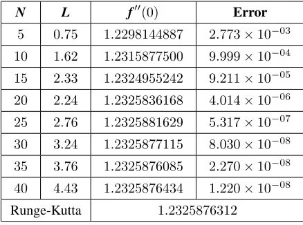
The approximations of thef00(0)computed by the RCC method for several values of N, with obtaining suitableLand their absolute errors have been shown in Table 1. The absolute errors have

been calculated with respect to the fourth-order Runge-Kutta solution. From Table 1, it is seen that

by increasing the number of the collocation points and obtaining suitableL, the absolute values of

Table 1: Numerical results for thef00(0)and their absolute errors for several values ofN

N L f00(0) Error

5 0.75 1.2298144887 2.773×10−03

10 1.62 1.2315877500 9.999×10−04

15 2.33 1.2324955242 9.211×10−05

20 2.24 1.2325836168 4.014×10−06

25 2.76 1.2325881629 5.317×10−07

30 3.24 1.2325877115 8.030×10−08

35 3.76 1.2325876085 2.270×10−08

40 4.43 1.2325876434 1.220×10−08 Runge-Kutta 1.2325876312

The logarithmic graph of the absolute coefficients|fi|of the rational Chebyshev functions in the

approximate solutions forN = 40by choosing suitableL = 4.43has been shown in Fig. 2. The graph shows the stability and convergence of the RCC method.

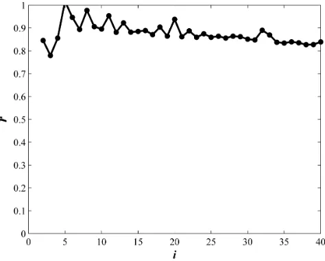
The exponential index of convergence,r, has been shown in Fig. 3 thatris calculated as

follow-ing:

r≡ lim

i→∞

log|log (|fi|)|

log (i)

from the Fig. 3, it is seen that r < 1 and according to Boyd [4], we conclude that the spectral approximation (14) has subgeometric convergence.

The comparison between the numerical solution given by Howarth [21] and approximation

solu-tion of the problem (7) with RCC method have been shown in Fig. 4. This figure displays that the

velocity profilef0(η) obtained by the RCC method agree with the boundary conditions (8). Also, between the results obtained by the RCC method and the Howarth values for all values ofη, a very

good adaption is seen.

The comparison of thef00(0)calculated by the present work with the values obtained by Wang [32], Howarth [21] and calculated by the fourth-order Runge-Kutta method has been given in Table

Figure 2 : Logarithmic graph of absolute coefficients|fi|of rational Chebyshev functions in approximate

solution forN= 40andL= 4.43

Figure 3 : The exponential index of convergencerversusi

In Table 3, the approximations of thef00(0) calculated by the RCC method together with their absolute errors for large numbers of the collocation points,N = 30,35,40 and different choices of Lfrom1to8, have been shown. It is seen that forN = 30whichN is a sufficiently large number, for all values ofLin this interval, the results are the same as that of Runge-Kutta to5digits decimal. Also forN = 35to6digits decimal and forN = 40to7digits decimal. So we can conclude that if N is chosen large enough, almost everyLin this interval achieves good results and not need to

Figure 4 : Graphs off(η),f0_(η)andf00_(η)calculated by the RCC method (N = 40,L= 4.43) and Howarth work [21]

9. CONCLUSION

In this study, we have applied an effective and accurate numerical technique that is known as the

RCC method to solve third-order nonlinear differential equation arising from the similarity solution

of two-dimensional Hiemenz flow of a viscous fluid impinging normal to an infinite plane situated

aty = 0. This technique is a powerful type of the collocation methods for solving the boundary value problems with semi-infinite domain without truncating it to a finite domain which employs the Table 2: A comparison of methods in [32], [21], the fourth-order Runge-Kutta and the present method

with the values forf00(0).

N L RCC Runge-Kutta Wang [32] Howarth [21]

25 2.76 1.2325881629

1.2325876312 1.232588 1.2326 30 3.24 1.2325877115

35 3.76 1.2325876085 40 4.43 1.2325876434

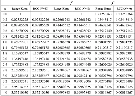
Table 4 shows the variations of f(η) approximated by the method proposed in this Letter for N = 40andL = 4.43, and those obtained by Howarth [21], Abbasbandy [3] and calculated by the

fourth-order Runge-Kutta method. Also, the results forf(η), f0_(η)andf00(η) have been shown in Table 5 byN = 40andL= 4.43and comparison have been made between the fourth-order Runge-Kutta’s solution and the presented numerical solution. This comparison shows that the RCC method

Table 3: Numerical results forf00(0)and their absolute errors for several values ofLandN.

N= 30 N= 35 N= 40

L f00(0) Error f00(0) Error f00(0) Error

1.0 1.23254296 4.47×10−05 _{1.23258300 4.63×10}−06 _{1.23258980 2.17×10}−06 1.5 1.23258242 5.21×10−06 _{1.23258675 8.83×10}−07 _{1.23258809 4.60×10}−07 2.0 1.23259151 3.88×10−06 _{1.23258700 6.31×10}−07 _{1.23258774 1.09×10}−07 2.5 1.23258579 1.84×10−06 _{1.23258794 3.11×10}−07 _{1.23258761 2.37×10}−08 3.0 1.23258897 1.34×10−06 _{1.23258751 1.17×10}−07 _{1.23258767 3.82×10}−08 3.5 1.23258668 9.50×10−07 _{1.23258778 1.46×10}−07 _{1.23258765 2.05×10}−08 4.0 1.23258794 3.10×10−07 _{1.23258754 9.02×10}−08 _{1.23258766 3.28×10}−08 4.5 1.23258823 6.02×10−07 _{1.23258772 9.43×10}−08 _{1.23258764 1.43×10}−08 5.0 1.23258704 5.95×10−07 _{1.23258769 5.64×10}−08 _{1.23258767 3.75×10}−08 5.5 1.23258724 3.86×10−07 _{1.23258756 6.69×10}−08 _{1.23258765 2.19×10}−08 6.0 1.23258827 6.35×10−07 _{1.23258766 3.44×10}−08 _{1.23258765 1.66×10}−08 6.5 1.23258832 6.89×10−07 _{1.23258775 1.24×10}−07 _{1.23258767 3.51×10}−08 7.0 1.23258739 2.45×10−07 _{1.23258766 3.22×10}−08 _{1.23258768 3.30×10}−08 7.5 1.23258667 9.58×10−07 _{1.23258754 8.57×10}−08 _{1.23258764 1.46×10}−08 8.0 1.23258697 6.58×10−07 _{1.23258758 5.40×10}−08 _{1.23258764 1.41×10}−08

Table 4: Approximation off(η)for present method, [2], [3] and Runge-Kutta method

η Howarth [21] Ref [3] Runge-Kutta RCC(N= 40)

0.0 0 0 0 0

0.2 0.0233 0.233355 0.0233222492 0.0233222570

0.6 0.1867 0.186715 0.1867009886 0.1867009935

1.0 0.4592 0.459236 0.4592270144 0.4592270171

1.4 0.7966 0.796657 0.7966517822 0.7966517836

1.8 1.1688 1.168855 1.1688554750 1.1688554755

2.0 1.3619 1.361968 1.3619741617 1.3619741619

2.4 1.7552 1.755238 1.7552538771 1.7552538766

2.8 2.1529 2.152965 2.1529965081 2.1529965067

Table 5: Comparison between RCC solution and Runge-Kutta solution forf(η), f0(η) andf00(η) withN = 40andL= 4.43.

f f0 f00

η Runge-Kutta RCC (N=40) Runge-Kutta RCC (N=40) Runge-Kutta RCC (N=40)

0.0 0 0 0 0 1.23258763 1.23258764

0.2 0.02332225 0.02332226 0.22661243 0.22661242 1.03445417 1.03445419

0.4 0.08805658 0.08805659 0.41445612 0.41445611 0.84632541 0.84632542

0.6 0.18670099 0.18670099 0.56628053 0.56628052 0.67517140 0.67517142

0.8 0.31242302 0.31242302 0.68593746 0.68593745 0.52513133 0.52513134

1.0 0.45922701 0.45922702 0.77786528 0.77786527 0.39801295 0.39801295

1.4 0.79665178 0.79665178 0.89680865 0.89680865 0.21100317 0.21100317

1.8 1.16885547 1.16885547 0.95683379 0.95683379 0.09996382 0.09996382

2.0 1.36197416 1.36197416 0.97321674 0.97321674 0.06582538 0.06582538

2.4 1.75525388 1.75525388 0.99054940 0.99054940 0.02602026 0.02602026

2.8 2.15299651 2.15299651 0.99704567 0.99704567 0.00904886 0.00904886

3.0 2.35255668 2.35255667 0.99842416 0.99842416 0.00507796 0.00507796

3.2 2.55232541 2.55232540 0.99918606 0.99918606 0.00275489 0.00275489

3.6 2.95214967 2.95214967 0.99980325 0.99980325 0.00073126 0.00073126

4.0 3.35210930 3.35210930 0.99995843 0.99995843 0.00016867 0.00016867 rational Chebyshev polynomials as the basis functions. Note that these basis functions have some

advantages: easy to compute, rapid convergence and completeness. This method reduces the solution

of a nonlinear ordinary differential equation to the solution of a system of algebraic equations. The

comparison between the numerical solution given by Howarth [21], Wang [32], Abbasbandy et al.

[3], the fourth-order Runge-Kutta solution and approximated by the current work, shows that RCC

method provides more accurate and numerically stable solutions than those obtained by other methods

REFERENCES

1. S. Abbasbandy, H. R. Ghehsareh and I. Hashim, An approximate solution of the MHD flow over a

non-linear stretching sheet by rational Chebyshev collocation method, U.P.B. Sci. Bull., Ser. A, 74 (2012),

47-58.

2. S. Abbasbandy, T. Hayat, H. R. Ghehsareh and A. Alsaedi, MHD Falkner-Skan flow of Maxwell fluid

by rational Chebyshev collocation method, Appl. Math. Mech., 34 (2013), 921-930.

3. S. Abbasbandy, K. Parand, S. Kazem and A. R. Sanaei Kia, A numerical approach on Hiemenz flow

problem using radial basis functions, Eur. Int. J. Industrial Math., 5(1) (2013), 65-73.

4. J. P. Boyd, Chebyshev and Fourier spectral methods, 2nd Ed., Springer, Berlin, (2000).

5. J. P. Boyd, Orthogonal rational functions on a semi-infinite interval, J. Comput. Phys., 70(1) (1987),

63-88.

6. J. P. Boyd, Spectral methods using rational basis functions on an infinite interval, J. Comput. Phys., 69

(1987), 112-142.

7. J. P. Boyd, The optimization of convergence for Chebyshev polynomial methods in an unbounded

do-main, J. Comput. Phys., 45 (1982), 43-79.

8. J. P. Boyd, C. Rangan and P. H. Bucksbaum, Pseudospectral methods on a semi-infinite interval with

application to the hydrogen atom: A comparison of the mapped Fourier-sine method with Laguerre

series and rational Chebyshev expansions, J. Comput. Phys., 188 (2003), 56-74.

9. C. Canuto, M. Y. Hussaini, A. Quarteroni and T. A. Zang, Spectral methods in fluids dynamics, Springer,

Berlin, (1990).

10. E. H. W. Cheng, M. N. Ozisik and J. C. William, Nonsteady three-dimensional stagnation point flow, J.

Appl. Mech., 38 (1971), 282-287.

11. A. Davey, Boundary layer flow at a saddle point of attachment, J. Fluid Mech., 10 (1961), 593-610.

12. D. Funaro, Computational aspects of pseudospectral Laguerre approximations, Appl. Numer. Math., 6

(1990), 447-457.

13. D. Funaro and O. Kavian, Approximation of some diffusion evolution equations in unbounded domains

by Hermite functions, Math. Comput., 57 (1991), 597-619.

14. H. R. Ghehsareh, B. Soltanalizadeh and S. A. Abbasbandy, A matrix formulation to the wave equation

with non-local boundary condition, Int. J. Comput. Math., 88 (2011), 1681-1696.

15. S. Goldstein, Modern developments in fluid dynamics, Oxford University Press, (1938).

16. B. Y. Guo, Error estimation of Hermite spectral method for nonlinear partial differential equations, Math.

Compt., 68(227) (1999), 1067-1078.

17. B. Y. Guo and J. Shen, Laguerre-Galerkin method for nonlinear partial differential equations on a

18. B. Y. Guo, J. Shen and Z. Q. Wang, Chebyshev rational spectral and pseudospectral methods on a

semi-infinite interval, Int. J. Numer. Meth. Engrg., 53 (2002), 65-84.

19. K. Hiemenz, Die Grenzschicht an einem in den gleichf¨ormigen Fl¨ussigkeitsstrom eingetauchten geraden

Kreiszylinder, Dingl. Polytech. J., 326 (1911), 321-410.

20. F. Homann, Der Einfluss grosser Z¨ahigkeit bei der Str¨omung um den Zylinder und um die Kugel, ZAMM

Z. Angew. Math. Mech., 16 (1936), 153-164.

21. L. Howarth, On the calculation of steady flow in the boundary layer near the surface of a cylinder in a

stream, Aeron. Res. Comm., Rep. Mem., 1632 (1934), 1-12.

22. L. Howarth, The boundary layer in three-dimensional flow. Part-II: The flow near a stagnation point,

Phil. Mag., Ser. VII, 42(335) (1951), 1433-1440.

23. Y. Maday, B. Pernaud-Thomas and H. Vandeven, Reappraisal of Laguerre type spectral methods, La

Rech. Aerospatiale, 6 (1985), 13-35.

24. K. Parand, Z. Delafkar and F. Bahari fard, Rational Chebyshev Tau method for solving natural

con-vection of Darcian fluid about a vertical full cone embedded in porous media whit a prescribed wall

temperature, World Academy of Science, Engineering and Technology, 5(8) (2011), 1186-1191.

25. K. Parand and M. Shahini, Rational Chebyshev pseudospectral approach for solving Thomas-Fermi

equation, Phys. Lett. A, 373 (2009), 210-213.

26. B. Sahoo and F. Labropulu, Steady Homann flow and heat transfer of an electrically conducting second

grade fluid, Comput. Math. Appl., 63 (2012), 1244-1255.

27. H. Schlichting, MHD Boundary layer theory, translate by J. Kestin, McGraw-Hill, (1968).

28. J. Shen, Stable and efficient spectral methods in unbounded domains using Laguerre functions, SIAM J.

Numer. Anal., 38(4) (2000), 1113-1133.

29. J. Shen and T. Tang, High order numerical methods and algorithms, Chinese Science Press, Beijing,

(2005).

30. J. Shen, T. Tang and L. L. Wang, Spectral Methods, Algorithms, Analysis and Applications, Springer,

Berlin, (2010).

31. H. Siyyam, Laguerre Tau methods for solving higher order ordinary differential equations, J. Comput.

Anal. Appl., 3(2) (2001), 173-182.

32. C. Y. Wang, Similarity stagnation point solutions of the Navier-Stokes equations- review and extension,